Python绘制气象实用地图(附代码和测试数据)

本文同步在MeteoAI和气象学家公众号推送。前面的推文对于常用的Python绘图工具都有了一些介绍，在这里就不赘述了。本文主要就以下几个方面：“中国区域绘图”、“包含南海”、“兰伯特投影带经纬度标签”、“基于salem的mask方法”、“进阶中国区域mask方法”、“进阶省份mask方法”。对日常的实用需求能够在一定程度上满足。

简单粗暴，Just show you my code!，细节暂不做过多分析，有问题可以探讨。数据、中文字体、地图shapefile文件、代码后文全部提供。使用建议，根据提示把缺失的库使用pip install xxx /conda install xxx /python setup.py install；安装完备，Python环境管理只推荐conda来统一管理。IDE推荐：PyCharm(有教育版)本地/服务器远程、Jupyter notebook。

---

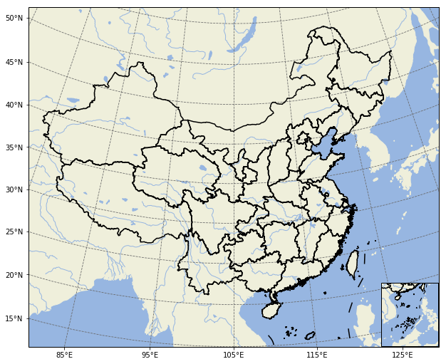
• 绘制兰勃脱投影的中国区域(包含南海子图)、
• Mask掉海洋部分的兰勃脱投影(包含南海子图)
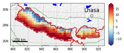
• 基于salem的白化
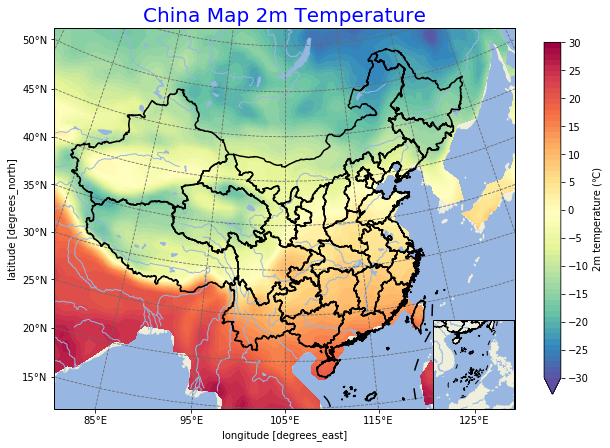
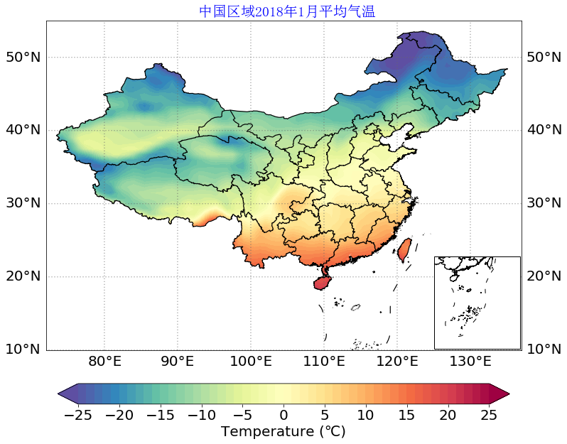
• 中国区域白化(包含南海子图)
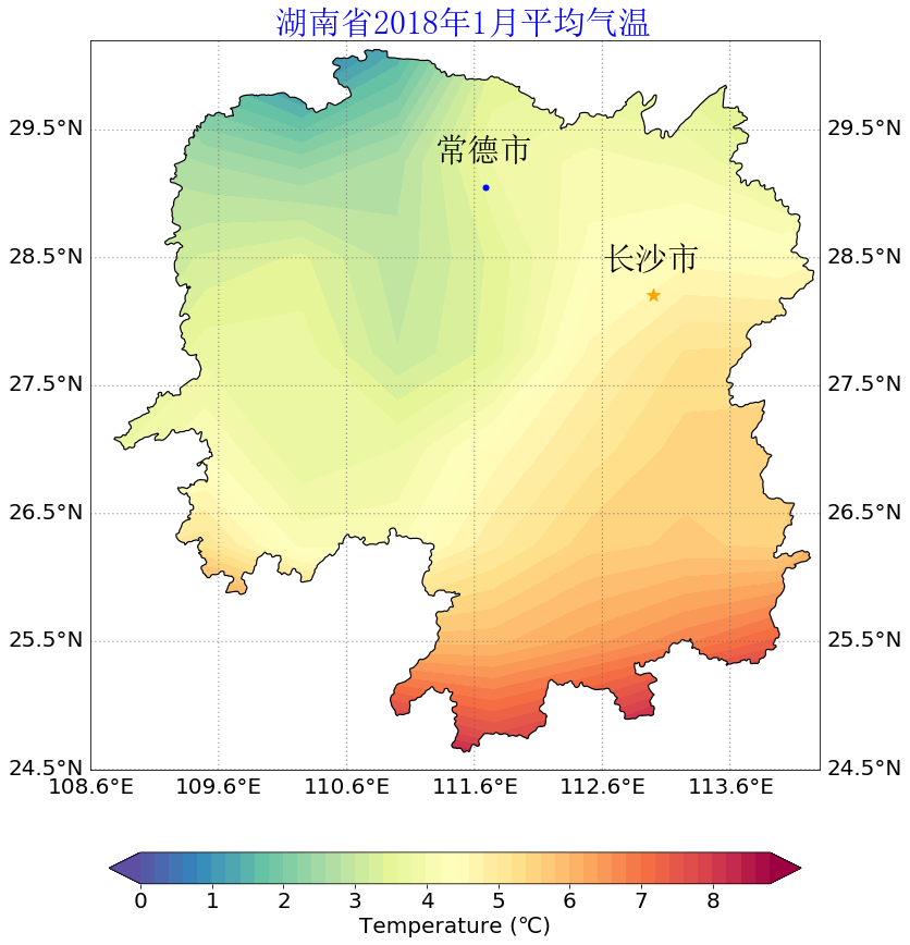
• 单独省份区域白化

---

绘制兰勃脱投影的中国区域(包含南海子图)代码；

import numpy as np
import xarray as xr
import matplotlib.pyplot as plt
import cartopy.crs as ccrs
import cartopy.feature as cfeature
from copy import copy
from cartopy.mpl.gridliner import LATITUDE_FORMATTER, LONGITUDE_FORMATTER
import shapely.geometry as sgeom



def find_side(ls, side):
    """
 Given a shapely LineString which is assumed to be rectangular, return the
 line corresponding to a given side of the rectangle.

 """
    minx, miny, maxx, maxy = ls.bounds
    points = {'left': [(minx, miny), (minx, maxy)],
              'right': [(maxx, miny), (maxx, maxy)],
              'bottom': [(minx, miny), (maxx, miny)],
              'top': [(minx, maxy), (maxx, maxy)],}
    return sgeom.LineString(points[side])

def lambert_xticks(ax, ticks):
    """Draw ticks on the bottom x-axis of a Lambert Conformal projection."""
    te = lambda xy: xy[0]
    lc = lambda t, n, b: np.vstack((np.zeros(n) + t, np.linspace(b[2], b[3], n))).T
    xticks, xticklabels = _lambert_ticks(ax, ticks, 'bottom', lc, te)
    ax.xaxis.tick_bottom()
    ax.set_xticks(xticks)
    ax.set_xticklabels([ax.xaxis.get_major_formatter()(xtick) for xtick in xticklabels])

def lambert_yticks(ax, ticks):
    """Draw ricks on the left y-axis of a Lamber Conformal projection."""
    te = lambda xy: xy[1]
    lc = lambda t, n, b: np.vstack((np.linspace(b[0], b[1], n), np.zeros(n) + t)).T
    yticks, yticklabels = _lambert_ticks(ax, ticks, 'left', lc, te)
    ax.yaxis.tick_left()
    ax.set_yticks(yticks)
    ax.set_yticklabels([ax.yaxis.get_major_formatter()(ytick) for ytick in yticklabels])

def _lambert_ticks(ax, ticks, tick_location, line_constructor, tick_extractor):
    """Get the tick locations and labels for an axis of a Lambert Conformal projection."""
    outline_patch = sgeom.LineString(ax.outline_patch.get_path().vertices.tolist())
    axis = find_side(outline_patch, tick_location)
    n_steps = 30
    extent = ax.get_extent(ccrs.PlateCarree())
    _ticks = []
    for t in ticks:
        xy = line_constructor(t, n_steps, extent)
        proj_xyz = ax.projection.transform_points(ccrs.Geodetic(), xy[:, 0], xy[:, 1])
        xyt = proj_xyz[..., :2]
        ls = sgeom.LineString(xyt.tolist())
        locs = axis.intersection(ls)
        if not locs:
            tick = [None]
        else:
            tick = tick_extractor(locs.xy)
        _ticks.append(tick[0])
    # Remove ticks that aren't visible: 
    ticklabels = copy(ticks)
    while True:
        try:
            index = _ticks.index(None)
        except ValueError:
            break
        _ticks.pop(index)
        ticklabels.pop(index)
    return _ticks, ticklabels


# Load the border data, CN-border-La.dat is downloaded from
# https://gmt-china.org/data/CN-border-La.dat
with open('CN-border-La.dat') as src:
    context = src.read()
    blocks = [cnt for cnt in context.split('>') if len(cnt) > 0]
    borders = [np.fromstring(block, dtype=float, sep=' ') for block in blocks]

    
# Set figure size
proj = ccrs.LambertConformal(central_longitude=105, central_latitude=90,
                             false_easting=400000, false_northing=400000)#,standard_parallels=(46, 49))

fig = plt.figure(figsize=[10, 8],frameon=True)


# Set projection and plot the main figure
ax = fig.add_axes([0.08, 0.05, 0.8, 0.94], projection=proj)
# Set figure extent
ax.set_extent([80, 130, 15, 55],crs=ccrs.PlateCarree())

# Plot border lines
for line in borders:
    ax.plot(line[0::2], line[1::2], '-', lw=1.5, color='k',
            transform=ccrs.Geodetic())

# Add ocean, land, rivers and lakes
ax.add_feature(cfeature.OCEAN.with_scale('50m'))
ax.add_feature(cfeature.LAND.with_scale('50m'))
ax.add_feature(cfeature.RIVERS.with_scale('50m'))
ax.add_feature(cfeature.LAKES.with_scale('50m'))


# *must* call draw in order to get the axis boundary used to add ticks:
fig.canvas.draw()

# Define gridline locations and draw the lines using cartopy's built-in gridliner:
# xticks = np.arange(80,130,10)
# yticks = np.arange(15,55,5)
xticks = [55, 65, 75, 85, 95, 105, 115, 125, 135, 145, 155, 165]
yticks = [0 , 5 , 10, 15, 20, 25 , 30 , 35 , 40 , 45 , 50 , 55 , 60 , 65]
ax.gridlines(xlocs=xticks, ylocs=yticks,linestyle='--',lw=1,color='dimgrey')

# Label the end-points of the gridlines using the custom tick makers:
ax.xaxis.set_major_formatter(LONGITUDE_FORMATTER) 
ax.yaxis.set_major_formatter(LATITUDE_FORMATTER)

lambert_xticks(ax, xticks)
lambert_yticks(ax, yticks)


#Plot South China Sea as a subfigure
sub_ax = fig.add_axes([0.754, 0.107, 0.14, 0.155],
                      projection=ccrs.LambertConformal(central_latitude=90,
                                                       central_longitude=115))
# Add ocean, land, rivers and lakes
sub_ax.add_feature(cfeature.OCEAN.with_scale('50m'))
sub_ax.add_feature(cfeature.LAND.with_scale('50m'))
sub_ax.add_feature(cfeature.RIVERS.with_scale('50m'))
sub_ax.add_feature(cfeature.LAKES.with_scale('50m'))
# Plot border lines
for line in borders:
    sub_ax.plot(line[0::2], line[1::2], '-', lw=1, color='k',
                transform=ccrs.Geodetic())
# Set figure extent
sub_ax.set_extent([105, 125, 0, 25],crs=ccrs.PlateCarree())

# Show figure
plt.savefig("China_nine_lines_lambert.png", dpi=500, bbox_inches='tight')
plt.show()

出图：

Mask掉海洋部分的兰勃脱投影(包含南海子图)

# https://gnss.help/2018/04/24/cartopy-gallery/index.html
# http://www.meteo.mcgill.ca/~cmccray/python.html
# https://www.jianshu.com/p/6506691f0788
# https://nbviewer.jupyter.org/gist/ajdawson/dd536f786741e987ae4e

import numpy as np
import os,sys
import xarray as xr
import matplotlib.pyplot as plt
import cartopy.crs as ccrs
import cartopy.feature as cfeature
from copy import copy
from cartopy.mpl.gridliner import LATITUDE_FORMATTER, LONGITUDE_FORMATTER
import shapely.geometry as sgeom


def find_side(ls, side):
    """
 Given a shapely LineString which is assumed to be rectangular, return the
 line corresponding to a given side of the rectangle.

 """
    minx, miny, maxx, maxy = ls.bounds
    points = {'left': [(minx, miny), (minx, maxy)],
              'right': [(maxx, miny), (maxx, maxy)],
              'bottom': [(minx, miny), (maxx, miny)],
              'top': [(minx, maxy), (maxx, maxy)],}
    return sgeom.LineString(points[side])

def lambert_xticks(ax, ticks):
    """Draw ticks on the bottom x-axis of a Lambert Conformal projection."""
    te = lambda xy: xy[0]
    lc = lambda t, n, b: np.vstack((np.zeros(n) + t, np.linspace(b[2], b[3], n))).T
    xticks, xticklabels = _lambert_ticks(ax, ticks, 'bottom', lc, te)
    ax.xaxis.tick_bottom()
    ax.set_xticks(xticks)
    ax.set_xticklabels([ax.xaxis.get_major_formatter()(xtick) for xtick in xticklabels])

def lambert_yticks(ax, ticks):
    """Draw ricks on the left y-axis of a Lamber Conformal projection."""
    te = lambda xy: xy[1]
    lc = lambda t, n, b: np.vstack((np.linspace(b[0], b[1], n), np.zeros(n) + t)).T
    yticks, yticklabels = _lambert_ticks(ax, ticks, 'left', lc, te)
    ax.yaxis.tick_left()
    ax.set_yticks(yticks)
    ax.set_yticklabels([ax.yaxis.get_major_formatter()(ytick) for ytick in yticklabels])

def _lambert_ticks(ax, ticks, tick_location, line_constructor, tick_extractor):
    """Get the tick locations and labels for an axis of a Lambert Conformal projection."""
    outline_patch = sgeom.LineString(ax.outline_patch.get_path().vertices.tolist())
    axis = find_side(outline_patch, tick_location)
    n_steps = 30
    extent = ax.get_extent(ccrs.PlateCarree())
    _ticks = []
    for t in ticks:
        xy = line_constructor(t, n_steps, extent)
        proj_xyz = ax.projection.transform_points(ccrs.Geodetic(), xy[:, 0], xy[:, 1])
        xyt = proj_xyz[..., :2]
        ls = sgeom.LineString(xyt.tolist())
        locs = axis.intersection(ls)
        if not locs:
            tick = [None]
        else:
            tick = tick_extractor(locs.xy)
        _ticks.append(tick[0])
    # Remove ticks that aren't visible: 
    ticklabels = copy(ticks)
    while True:
        try:
            index = _ticks.index(None)
        except ValueError:
            break
        _ticks.pop(index)
        ticklabels.pop(index)
    return _ticks, ticklabels


# Load the border data, CN-border-La.dat is downloaded from
# https://gmt-china.org/data/CN-border-La.dat
with open('CN-border-La.dat') as src:
    context = src.read()
    blocks = [cnt for cnt in context.split('>') if len(cnt) > 0]
    borders = [np.fromstring(block, dtype=float, sep=' ') for block in blocks]

    
# Set figure size
proj = ccrs.LambertConformal(central_longitude=105, central_latitude=90,
                             false_easting=400000, false_northing=400000)#,standard_parallels=(46, 49))

fig = plt.figure(figsize=[10, 8],frameon=True)

# Set projection and plot the main figure
ax = fig.add_axes([0.08, 0.05, 0.8, 0.94], projection=proj)
# Set figure extent
ax.set_extent([80, 130, 15, 55],crs=ccrs.PlateCarree())
# ax.set_title('ChinaChinaChinaChinaChinaChinaChinaChinaChinaChina',fontsize=20)       
# Plot border lines
for line in borders:
    ax.plot(line[0::2], line[1::2], '-', lw=1.5, color='k',
            transform=ccrs.Geodetic())

# Add ocean, land, rivers and lakes
ax.add_feature(cfeature.OCEAN.with_scale('50m'))
ax.add_feature(cfeature.LAND.with_scale('50m'))
ax.add_feature(cfeature.RIVERS.with_scale('50m'))
ax.add_feature(cfeature.LAKES.with_scale('50m'))


# *must* call draw in order to get the axis boundary used to add ticks:
fig.canvas.draw()

# Define gridline locations and draw the lines using cartopy's built-in gridliner:
# xticks = np.arange(80,130,10)
# yticks = np.arange(15,55,5)
xticks = [55, 65, 75, 85, 95, 105, 115, 125, 135, 145, 155, 165]
yticks = [0 , 5 , 10, 15, 20, 25 , 30 , 35 , 40 , 45 , 50 , 55 , 60 , 65]
ax.gridlines(xlocs=xticks, ylocs=yticks,linestyle='--',lw=1,color='dimgrey')

# Label the end-points of the gridlines using the custom tick makers:
ax.xaxis.set_major_formatter(LONGITUDE_FORMATTER) 
ax.yaxis.set_major_formatter(LATITUDE_FORMATTER)

# https://stackoverflow.com/questions/30030328/correct-placement-of-colorbar-relative-to-geo-axes-cartopy
# ax.set_aspect('auto', adjustable=None)

lambert_xticks(ax, xticks)
lambert_yticks(ax, yticks)

#Plot South China Sea as a subfigure
sub_ax = fig.add_axes([0.592, 0.189, 0.14, 0.155],
                      projection=ccrs.LambertConformal(central_latitude=90,
                                                       central_longitude=115))
# Add ocean, land, rivers and lakes
sub_ax.add_feature(cfeature.OCEAN.with_scale('50m'))
sub_ax.add_feature(cfeature.LAND.with_scale('50m'))
sub_ax.add_feature(cfeature.RIVERS.with_scale('50m'))
sub_ax.add_feature(cfeature.LAKES.with_scale('50m'))
# Plot border lines
for line in borders:
    sub_ax.plot(line[0::2], line[1::2], '-', lw=1, color='k',
                transform=ccrs.Geodetic())
# Set figure extent
sub_ax.set_extent([105, 125, 0, 25],crs=ccrs.PlateCarree())

def mask(ds, label='land'):
    landsea = xr.open_dataset('landsea.nc')
    landsea = landsea['LSMASK']
    # --ds和地形数据分辨率不一致，需将地形数据插值
    landsea = landsea.interp(lat=ds.latitude.values, lon=ds.longitude.values)
    # --利用地形掩盖海陆数据
    ds.coords['mask'] = (('latitude', 'longitude'), landsea.values)
    print(ds.mask)
    if label == 'land':
        ds = ds.where(ds.mask < 0.8) #可以尝试调整default：0.8
    elif label == 'ocean':
        ds = ds.where(ds.mask > 0.3) #可以尝试调整default：0.2
    return ds

ds = xr.open_dataset('EC-Interim_monthly_2018.nc')
lat = ds.latitude
lon = ds.longitude
time = ds.time
temp = (ds['t2m'] - 273.15) # 把温度转换为℃
# 区域选择
lon_range = lon[(lon>60) & (lon<150)]
lat_range = lat[(lat>10) & (lat<60)]
temp_region = temp.sel(longitude=lon_range, latitude=lat_range, time='2018-02-01')
temp_mask = mask(temp_region, 'ocean')
# 设置colorbar 
#get size and extent of axes:

cbar_kwargs = {
    'orientation': 'vertical',
    'label': '2m temperature (℃)',
    'shrink': 0.8,
    'ticks': np.arange(-30, 30 + 5, 5),
    'pad': 0.05,
    'shrink': 0.65
}


# 画图
levels = np.arange(-30, 30 + 1, 1)
temp_mask.plot.contourf(ax=ax, levels=levels, cmap='Spectral_r',
                        cbar_kwargs=cbar_kwargs, transform=ccrs.PlateCarree())
# 设置标题的在代码中放置的位置很关键，注意不要放置在小图上或者新建画框了。
ax.set_title('China Map 2m Temperature',color='blue',fontsize= 20)

# Save & Show figure
# (filename, extension) = os.path.splitext(os.path.basename(sys.argv[0]))
plt.savefig("land_sea_mask_simple_lambert.png", dpi=500, bbox_inches='tight')
plt.show()

出图：

基于salem的白化

import salem
import matplotlib.pyplot as plt
from salem.utils import get_demo_file
ds = salem.open_xr_dataset(get_demo_file('wrfout_d01.nc'))
t2 = ds.T2.isel(Time=2)
# t2.salem.quick_map()
t2_sub = t2.salem.subset(corners=((77., 20.), (97., 35.)), crs=salem.wgs84)
# t2_sub.salem.quick_map()
shdf = salem.read_shapefile(get_demo_file('world_borders.shp'))
shdf = shdf.loc[shdf['CNTRY_NAME'].isin(['Nepal', 'Bhutan'])]  # GeoPandas' GeoDataFrame
t2_sub = t2_sub.salem.subset(shape=shdf, margin=2)  # add 2 grid points
# t2_sub.salem.quick_map()
t2_roi = t2_sub.salem.roi(shape=shdf)
# t2_roi.salem.quick_map()

# Change the country borders
smap = t2_roi.salem.get_map(data=t2_roi-273.15, cmap='RdYlBu_r', vmin=-14, vmax=18)
_ = smap.set_topography(get_demo_file('himalaya.tif'))
smap.set_shapefile(shape=shdf, color='grey', linewidth=3)
smap.set_shapefile(countries=True, color='C3', linewidths=2)

# Add oceans and lakes
smap.set_shapefile(oceans=True)
smap.set_shapefile(rivers=True,linewidths=0.8,color='green')
smap.set_shapefile(lakes=True, facecolor='blue', edgecolor='blue')

# Change the lon-lat countour setting
smap.set_lonlat_contours(add_ytick_labels=True, interval=2, linewidths=0.5,
                         linestyles='--', colors='grey')

# Add a scalebar (experimental)
smap.set_scale_bar(location=(0.10, 0.10), add_bbox=False)

smap.set_points(91.1, 29.6)
smap.set_text(90.0, 30.1, 'Lhasa', fontsize=17)

smap.visualize()
plt.savefig("Himalayas_mask.png", dpi=500, bbox_inches='tight')
plt.show()

出图：

中国区域白化(包含南海子图)

#https://regionmask.readthedocs.io/en/stable/defined_landmask.html
#coding=utf-8
from mpl_toolkits.basemap import Basemap
from matplotlib.path import Path
from matplotlib.patches import PathPatch
import matplotlib.pyplot as plt
from osgeo import gdal
import numpy as np
import cartopy.crs as ccrs
import shapefile
import xarray as xr
import matplotlib as mpl
from matplotlib.font_manager import FontProperties
import netCDF4 as nc
from cartopy.mpl.gridliner import LONGITUDE_FORMATTER, LATITUDE_FORMATTER

import matplotlib
ZHfont = matplotlib.font_manager.FontProperties(fname='/Users/zhpfu/Documents/fonts/SimSun.ttf')

plt.rcParams.update({'font.size':20})


fig = plt.figure(figsize=[12,18]) 
ax = fig.add_subplot(111)



sf = shapefile.Reader("country1")
for shape_rec in sf.shapeRecords():
    if shape_rec.record[2] == 'China':#Hunan Sheng
        vertices = []
        codes = []
        pts = shape_rec.shape.points
        prt = list(shape_rec.shape.parts) + [len(pts)]
        for i in range(len(prt) - 1):
            for j in range(prt[i], prt[i+1]):
                vertices.append((pts[j][0], pts[j][1]))
            codes += [Path.MOVETO]
            codes += [Path.LINETO] * (prt[i+1] - prt[i] -2)
            codes += [Path.CLOSEPOLY]
        clip = Path(vertices, codes)
        clip = PathPatch(clip, transform=ax.transData)


        
def makedegreelabel(degreelist):
    labels=[str(x)+u'°E' for x in degreelist]
    return labels


ds = xr.open_dataset('EC-Interim_monthly_2018.nc')
lat = ds.latitude
lon = ds.longitude
data = (ds['t2m'][0,::-1,:] - 273.15) # 把温度转换为℃   [0,::-1,:]表示第一个时次、纬度反向

# ncdata=nc.Dataset('EC-Interim_monthly_2018.nc')
# data=ncdata.variables['t2m'][0,::-1,:] - 273.15 # 把温度转换为℃ 
# lat=ncdata.variables['latitude'][:]
# lon=ncdata.variables['longitude'][:]

nx=data.shape[1]
ny=data.shape[0]
               
m = Basemap(llcrnrlon=72.0,
    llcrnrlat=10.0,
    urcrnrlon=137.0,
    urcrnrlat=55.0,
    resolution = None, 
    projection = 'cyl')


cbar_kwargs = {
    'orientation': 'horizontal',
    'label': 'Temperature (℃)',
    'shrink': 0.02,
    'ticks': np.arange(-25, 25 + 1, 5),
    'pad': -0.28,
    'shrink': 0.95
}


# 画图
levels = np.arange(-25, 25 + 1, 1)   
cs = data.plot.contourf(ax=ax,levels=levels,cbar_kwargs=cbar_kwargs, cmap='Spectral_r')
# 设置标题的在代码中放置的位置很关键，注意不要放置在小图上或者新建画框了。

m.readshapefile('bou2_4l','China Map',color='k',linewidth=1.2)

for contour in cs.collections:
        contour.set_clip_path(clip)

        
# draw parallels and meridians.
# label parallels on right and top
# meridians on bottom and left
# http://code.activestate.com/recipes/578399-an-alternative-way-to-draw-parallels-and-meridians/
parallels = np.arange(10,55,10)
# labels = [left,right,top,bottom]
m.drawparallels(parallels,labels=[True,True,True,True],color='dimgrey',dashes=[1, 3])  # ha= 'right'
meridians = np.arange(70,135,10)
m.drawmeridians(meridians,labels=[True,True,False,True],color='dimgrey',dashes=[1, 3])


#http://xarray.pydata.org/en/stable/plotting.html
plt.ylabel('')    #Remove the defult  lat / lon label  
plt.xlabel('')        
           

plt.rcParams.update({'font.size':30})
ax.set_title(u' 中国区域2018年1月平均气温',color='blue',fontsize= 25 ,fontproperties=ZHfont) # 2m Temperature


plt.rcParams.update({'font.size':20})
        
with open('CN-border-La.dat') as src:
    context = src.read()
    blocks = [cnt for cnt in context.split('>') if len(cnt) > 0]
    borders = [np.fromstring(block, dtype=float, sep=' ') for block in blocks]
    
#Plot South China Sea as a subfigure
sub_ax = fig.add_axes([0.758, 0.249, 0.14, 0.155],
                      projection=ccrs.LambertConformal(central_latitude=90,
                                                       central_longitude=115))
# Plot border lines
for line in borders:
    sub_ax.plot(line[0::2], line[1::2], '-', lw=1, color='k',
                transform=ccrs.Geodetic())
# Set figure extent
sub_ax.set_extent([106, 127, 0, 25],crs=ccrs.PlateCarree())        

        
# Save & Show figure
plt.savefig("China_mask_T2m.png", dpi=300, bbox_inches='tight')
plt.show()

出图：

单独省份区域白化

#https://basemaptutorial.readthedocs.io/en/latest/clip.html
#coding=utf-8
from mpl_toolkits.basemap import Basemap
from matplotlib.path import Path
from matplotlib.patches import PathPatch
import matplotlib.pyplot as plt
from osgeo import gdal
import numpy as np
import cartopy.crs as ccrs
import shapefile
import matplotlib as mpl
import xarray as xr
from matplotlib.font_manager import FontProperties
import netCDF4 as nc
from cartopy.mpl.gridliner import LONGITUDE_FORMATTER, LATITUDE_FORMATTER

import matplotlib
ZHfont = matplotlib.font_manager.FontProperties(fname='/Users/zhpfu/Documents/fonts/SimSun.ttf')


plt.rcParams.update({'font.size': 20})

# plt.clf()
fig = plt.figure(figsize=[12,18]) 

# fig = plt.figure(figsize=(16,8.5),dpi=300)# figsize=(16,9.6)   
ax = fig.add_subplot(111)

 
# set the projection to PlateCarree
# proj = ccrs.PlateCarree()
# ax = fig.add_subplot(1, 1, 1,projection = proj)

# ax=fig.add_axes([.2,.2,.6,.68]) #[*left*, *bottom*, *width*,*height*]

sf = shapefile.Reader("national_provinces_shp/hunan")
for shape_rec in sf.shapeRecords():
    if shape_rec.record[2] == 'Hunan Sheng':#Hunan Sheng
        vertices = []
        codes = []
        pts = shape_rec.shape.points
        prt = list(shape_rec.shape.parts) + [len(pts)]
        for i in range(len(prt) - 1):
            for j in range(prt[i], prt[i+1]):
                vertices.append((pts[j][0], pts[j][1]))
            codes += [Path.MOVETO]
            codes += [Path.LINETO] * (prt[i+1] - prt[i] -2)
            codes += [Path.CLOSEPOLY]
        clip = Path(vertices, codes)
        clip = PathPatch(clip, transform=ax.transData)


        
def makedegreelabel(degreelist):
    labels=[str(x)+u'°E' for x in degreelist]
    return labels


ds = xr.open_dataset('EC-Interim_monthly_2018.nc')
lat = ds.latitude
lon = ds.longitude
data = (ds['t2m'][0,::-1,:] - 273.15) # 把温度转换为℃

nx=data.shape[1]
ny=data.shape[0]


# Hunan Province region = [108.6,114.3,24.5,30.2] # [west,east,south,north]

m = Basemap(llcrnrlon=108.6,
    llcrnrlat=24.5,
    urcrnrlon=114.3,
    urcrnrlat=30.2,
    resolution = None, 
    projection = 'cyl')


cbar_kwargs = {
    'orientation': 'horizontal',
    'label': 'Temperature (℃)',
    'shrink': 0.02,
    'ticks': np.arange(0, 10 + 1, 1),
    'pad': -0.01,
    'shrink': 0.95
}



# 画图
levels = np.arange(0, 8 + 1, 0.2)   
cs = data.plot.contourf(ax=ax,levels=levels,cbar_kwargs=cbar_kwargs, cmap='Spectral_r')
# 设置标题的在代码中放置的位置很关键，注意不要放置在小图上或者新建画框了。

m.readshapefile('national_provinces_shp/hunan','Hunan Map',color='k',linewidth=1.2)

for contour in cs.collections:
        contour.set_clip_path(clip)

# draw parallels and meridians.
# label parallels on right and top
# meridians on bottom and left
# http://code.activestate.com/recipes/578399-an-alternative-way-to-draw-parallels-and-meridians/
parallels = np.arange(24.5,30.2,1.0)
# labels = [left,right,top,bottom]
m.drawparallels(parallels,labels=[True,True,True,True],color='dimgrey',dashes=[1, 3])  # ha= 'right'
meridians = np.arange(108.6,114.3,1.0)
m.drawmeridians(meridians,labels=[True,True,False,True],color='dimgrey',dashes=[1, 3])


#http://xarray.pydata.org/en/stable/plotting.html
plt.ylabel('')    #Remove the defult  lat / lon label  
plt.xlabel('')


plt.rcParams.update({'font.size':30})
ax.set_title(u' 湖南省2018年1月平均气温',color='blue',fontsize= 25 ,fontproperties=ZHfont) # 2m Temperature

bill0 = 111.69
tip0  =  29.05
plt.scatter(bill0, tip0,marker='.',s=100 ,color ="blue")


bill2 =  113.0
tip2  = 28.21
plt.scatter(bill2, tip2,marker='*',s=150 ,color ="orange" )

plt.rcParams.update({'font.size':30})
plt.text(bill0-0.4, tip0+0.2, u"常德市", fontsize= 20 ,fontproperties=ZHfont)
plt.text(bill2-0.4, tip2+0.2, u"长沙市", fontsize= 20 ,fontproperties=ZHfont)

# Save & Show figure
plt.savefig("Hunan_mask_T2m.png", dpi=300, bbox_inches='tight')
plt.show()

出图：

测试数据和代码：链接:https://pan.baidu.com/s/18R6RWYhi5p_wMbMrdKzw2g 密码:jwil

参考：

链接.1
链接.2
链接.3
链接.4
链接.5
链接.6
链接.7
链接.8

有任何问题都欢迎交流探讨，共同学习进步！