如何用NCL处理风云4A/MODIS卫星数据?

本文在『气象学家』同步推送传送门;读取和处理了两种FY-4A和MODIS卫星数据,进行相关产品的绘图,插值为不同分辨率经纬度格点数据并保存为nc格式文件。抛砖引玉,不做更深入的分析。

00.前言介绍

工具:NCL、相关底图包
配料:风云4A数据FY4_AGRI_L2 OLR产品、MOD06_L2产品
方法:ESMF_regrid
成品:中国区域图、经纬度格点数据(e.g. , 0.1°*0.1°)

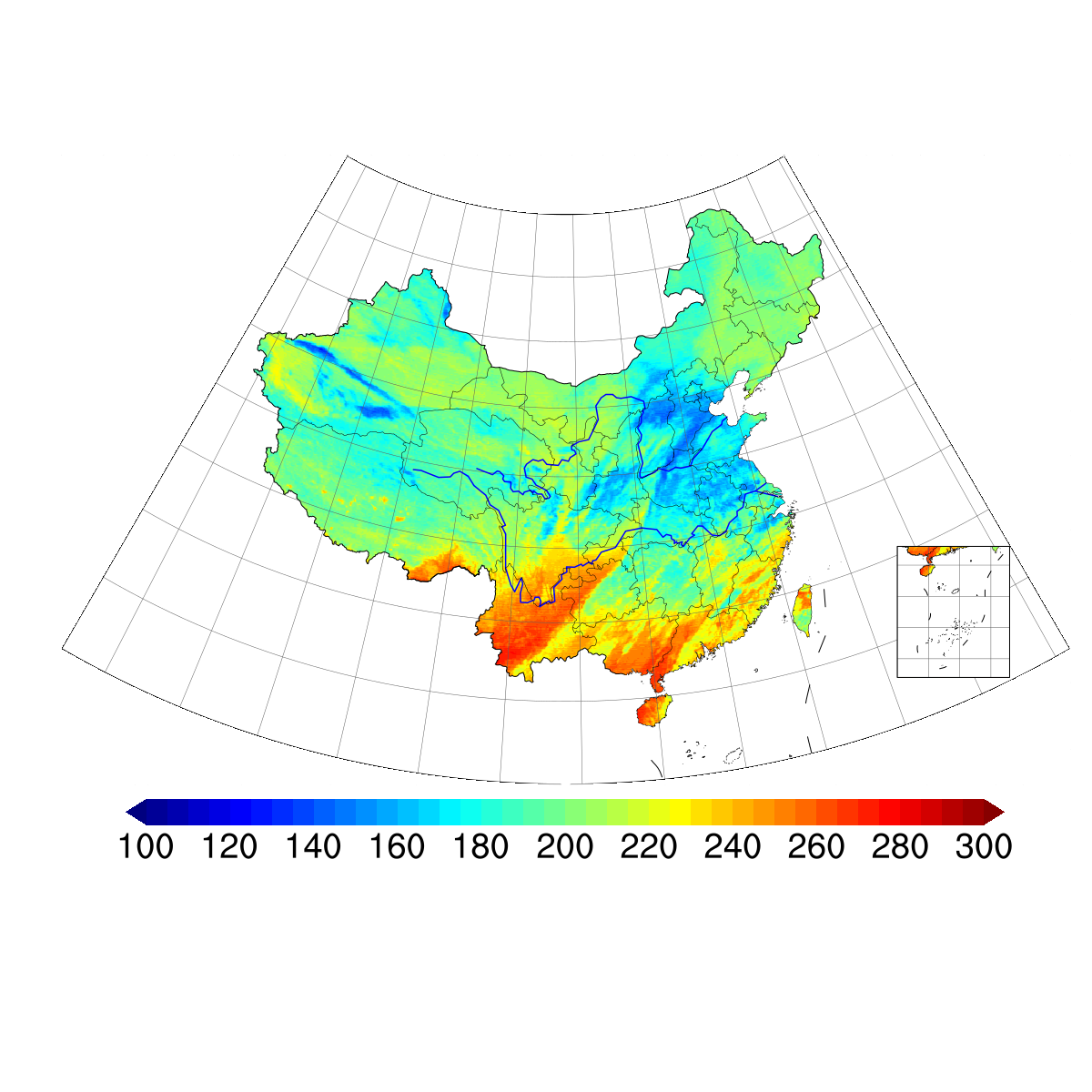
01.中国区域FY4_AGRI_L2 OLR原始数据Lambert投影绘图和脚本

1
2
3
4
5
6
7
8
9
10
11
12
13
14
15
16
17
18
19
20
21
22
23
24
25
26
27
28
29
30
31
32
33
34
35
36
37
38
39
40
41
42
43
44
45
46
47
48
49
50
51
52
53
54
55
56
57
58
59
60
61
62
63
64
65
66
67
68
69
70
71
72
73
74
75
76
77
78
79
80
81
82
83
84
85
86
87
88
89
90
91
92
93
94
95
96
97
98
99
100
101
102
103
104
105
106
107
108
109
110
111
112
113
114
115
116
117
118
119
120
121
122
123
124
125
126
127
128
129
130
131
132
133
134
135
136
137
138
139
140
141
142
143
144
145
146
147
148
149
150
151
152
153
154
155
156
157
158
159
160
161
162
163
164
165
166
167
168
169
170
171
172
173
174
175
176
177
178
179
180
181
182
183
184
185
186
187
188
189
190
191
192
193
194
195
196
197
198
199
200
201
202
203
204
205
206
207
208
209
210
211
212
213
214
215
216
217
218
; =============================================================================
; Author: Gavin | Affiliation: NJU
; Email : Zhpfu.atm@gmail.com
; Last modified: 2018-06-18 10:43
; Filename: FY4A_read_plot_latlon2d_Lambert.ncl
; Description: Read FY4A full disc data;
; Take OLR for example;
; Mapping to specific area;
; Plotting China area with China's nine-dash;
; Choosing Lambert Map Projections;
; To Be Determined(TBD):
;
; =============================================================================

; =============================================================================
; Given a start time and a title, this procedure calls get_cpu_time()
; to get the end_time, then prints "elapsed time" information.
; =============================================================================
procedure print_elapsed_time(start_time,title)
local end_time
begin

end_time = get_cpu_time()
print("======================================================================")
print(title + " elapsed time = " + (end_time-start_time) + " CPU seconds.")
print("======================================================================")
end

; =============================================================================
; ===================================MAIN======================================
; =============================================================================
start_time = get_cpu_time()

fpath = "/Users/zhpfu/Downloads/DATA_MAC/00_FY_satellite/"
fname = "FY4A-_AGRI--_N_DISK_1047E_L2-_OLR-_MULT_NOM_20180104000000_20180104001459_4000M_V0001.NC"
f1 = addfile(fpath+fname,"r")
geohdf= "FY4A_OBI_4000M_NOM_LATLON.HDF"
f2 = addfile(fpath+geohdf,"r")

lon2d = f2->Lon(:,:)
lat2d = f2->Lat(:,:)

; Set default value
; 65534 is the area out of Earth
lon2d@_FillValue = 65534
lat2d@_FillValue = 65534

if (any(ismissing(ndtooned(lon2d)))) then
print("Missing longitude coordinates detected")
end if

if (any(ismissing(ndtooned(lat2d)))) then
print("Missing latitude coordinates detected")
end if

; Set the specific area to plot
minlat = 15.
maxlat = 55.
minlon = 72.
maxlon = 136.

olr =short2flt(f1->OLR)
olr@_FillValue = 32766

; Add the attributes
lat2d@units = "degrees_north"
lon2d@units = "degrees_east"
olr@lat2d = lat2d
olr@lon2d = lon2d
olr@units = "W/M2"
olr@coordinates = "lat2d lon2d"

; =============================================================================
; ================================plot=========================================
; =============================================================================

wks_type = "png"
wks_type@wkWidth = 1200
wks_type@wkHeight = 1200

wks = gsn_open_wks(wks_type,"FY4A_OLR_plot_latlon2d_Lambert") ; send graphics to PNG file
gsn_define_colormap(wks, "NCV_jet") ;MPL_jet

; colors = (/ (/1,1,1/),\
; (/0,0,0/),\
; (/1,1,1/),\
; (/0.647,0.953,0.553/),\
; (/0.239,0.725,0.247/), \
; (/0.388,0.722,0.976/), \
; (/0,0,0.996/),\
; (/0.953,0.020,0.933/),\
; (/0.506,0,0.251/)/)

; gsn_define_colormap(wks,colors)


res = True ; plot mods desired
res@gsnMaximize = True ; maximize plot in frame
res@gsnDraw = False
res@gsnFrame = False
res@mpProjection = "LambertConformal" ; choose projection
res@gsnSpreadColors = True ; Use full color map

res@sfXArray = lon2d
res@sfYArray = lat2d


res@cnFillOn = True ; color fill
res@cnFillMode = "RasterFill" ; Raster mode is much faster
res@cnRasterSmoothingOn = True
; res@cnFillPalette = "gui_default"
res@cnLinesOn = False ; and uses less memory.
res@cnLineLabelsOn = False
res@trGridType = "TriangularMesh" ; Caution!!! can not ignore!

; =============================================================================
; set for map
res@mpLimitMode = "LatLon"
res@mpMinLatF = minlat
res@mpMaxLatF = maxlat
res@mpMinLonF = minlon
res@mpMaxLonF = maxlon

res@mpFillOn = True
res@mpDataSetName = "/Users/zhpfu/Downloads/DATA_MAC/00_FY_satellite/FY4A/NCL-Chinamap/database/Earth..4"
res@mpDataBaseVersion = "MediumRes" ; or "Ncarg4_1"
res@mpAreaMaskingOn = True
res@mpMaskAreaSpecifiers = (/"China"/)
res@mpOutlineSpecifiers = (/"China","China:Provinces"/)


res@mpLandFillColor = "white"
res@mpInlandWaterFillColor = "white"
res@mpOceanFillColor = "white"
res@mpFillBoundarySets = "NoBoundaries"
res@mpOutlineBoundarySets = "NoBoundaries"
res@mpNationalLineColor = "black"
res@mpProvincialLineColor = "black"
res@mpGeophysicalLineColor = "black"
res@mpNationalLineThicknessF = 2
res@mpProvincialLineThicknessF = 1

res@mpGridAndLimbOn = "True"
res@mpGridAndLimbDrawOrder = "Draw"
; res@mpGridMaskMode = "MaskLand"
res@mpGridSpacingF = 5.0
res@mpGridLineColor = "Grey37"
; =============================================================================
; set for the plot

res@cnFillDrawOrder = "PreDraw"
res@cnLevelSelectionMode = "ManualLevels" ; set manual contour levels
res@cnMinLevelValF = 100;min(olr) ; set min contour level
res@cnMaxLevelValF = 300;max(olr) ; set max contour level
res@cnLevelSpacingF = 5.0 ; set contour spacing

res@gsnAddCyclic = False

; res@tmXTOn = True
; res@tmYROn = True

res@lbOrientation = "Horizontal" ; vertical labelbar
res@pmTickMarkDisplayMode= "Always"
; res@pmLabelBarOrthogonalPosF = 0.00 ; Move labelbar up
; res@pmLabelBarParallelPosF = 0.00 ; Move labelbar Right
res@pmLabelBarWidthF = 0.35
res@pmLabelBarHeightF = 0.035
res@lbLabelFontHeightF = 0.005
res@lbPerimOn = False

res@lbLabelAutoStride = True ; Clean up labelbar labels.
res@lbBoxLinesOn = False ; No labelbar box lines.
res@lbLabelFontHeightF = 0.01 ; make labels smaller ( default=0.02 )
res@lbBoxEndCapStyle = "TriangleBothEnds" ; set the two-end triangle
res@tiXAxisString = ""
res@tiYAxisString = ""
res@gsnStringFontHeightF = 0.012
res@gsnLeftString = "";"OLR"
res@gsnRightString = "";"W/m~S~2~E~" ;"W/m2"
res@gsnMaskLambertConformal = True ; turn on lc masking
; res@gsnMaskLambertConformalOutlineOn = False ; turns off outline
plot = gsn_csm_contour_map(wks,olr,res) ; create plot

; =============================================================================
; add South China Sea
nhres = res
nhres@gsnMaximize = False
nhres@vpHeightF = 0.12
nhres@vpWidthF = 0.12

nhres@mpMinLatF = 2
nhres@mpMaxLatF = 23
nhres@mpMinLonF = 105
nhres@mpMaxLonF = 123
nhres@lbLabelBarOn = False
nhres@tmXBOn = False
nhres@tmXTOn = False
nhres@tmYLOn = False
nhres@tmYROn = False
nhres@gsnLeftString = ""
nhres@gsnRightString = ""
nhres@mpProjection = "CylindricalEquidistant" ; choose projection
map_nanhai = gsn_csm_contour_map(wks,olr,nhres)
adres = True
adres@amParallelPosF = 0.44 ;0.499 ; -0.5 is the left edge of the plot.
adres@amOrthogonalPosF = 0.33 ;0.50 ; -0.5 is the top edge of the plot.
adres@amJust = "BottomRight"
plotnh = gsn_add_annotation(plot,map_nanhai,adres)

; add Changjiang and Huanghe river
river = True
river@gsLineThicknessF = 3.0
river@gsLineColor = "blue"
plotrv = gsn_add_shapefile_polylines(wks,plot,"/Users/zhpfu/Downloads/DATA_MAC/00_FY_satellite/FY4A/NCL-Chinamap/cnmap_NetCDF/river.nc",river)
draw(plot)
frame(wks)

print_elapsed_time(start_time,"Game Over >>>>>>>")

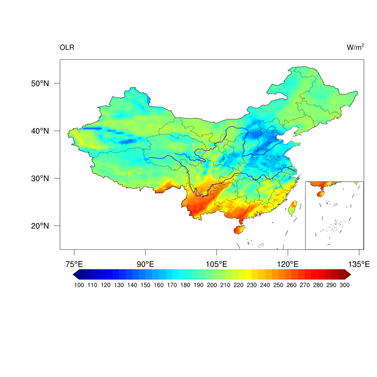
02.中国区域FY4_AGRI_L2 OLR原始数据经纬度网格投影绘图和脚本

1
2
3
4
5
6
7
8
9
10
11
12
13
14
15
16
17
18
19
20
21
22
23
24
25
26
27
28
29
30
31
32
33
34
35
36
37
38
39
40
41
42
43
44
45
46
47
48
49
50
51
52
53
54
55
56
57
58
59
60
61
62
63
64
65
66
67
68
69
70
71
72
73
74
75
76
77
78
79
80
81
82
83
84
85
86
87
88
89
90
91
92
93
94
95
96
97
98
99
100
101
102
103
104
105
106
107
108
109
110
111
112
113
114
115
116
117
118
119
120
121
122
123
124
125
126
127
128
129
130
131
132
133
134
135
136
137
138
139
140
141
142
143
144
145
146
147
148
149
150
151
152
153
154
155
156
157
158
159
160
161
162
163
164
165
166
167
168
169
170
171
172
173
174
175
176
177
178
179
180
181
182
183
184
185
186
187
188
189
190
191
192
193
194
195
196
197
198
199
200
201
202
203
204
205
206
207
208
209
210
; =============================================================================
; Author: Gavin | Affiliation: NJU
; Email : Zhpfu.atm@gmail.com
; Last modified: 2018-06-18 01:15
; Filename: FY4A_read_plot_latlon2d_to_rectilinear_grid.ncl
; Description: Read FY4A full disc data;
; Take OLR for example;
; Mapping to specific area;
; Plotting China area with China's nine-dash;
; Choosing different Map Projections;
; To Be Determined(TBD):
; 问题:需要局部微调,经纬度刻度最好四周都有;投影方式暂时只有圆柱等距投影
; Cylindrical Equidistant Projection;
; =============================================================================

; =============================================================================
; Given a start time and a title, this procedure calls get_cpu_time()
; to get the end_time, then prints "elapsed time" information.
; =============================================================================
procedure print_elapsed_time(start_time,title)
local end_time
begin

end_time = get_cpu_time()
print("======================================================================")
print(title + " elapsed time = " + (end_time-start_time) + " CPU seconds.")
print("======================================================================")
end

; =============================================================================
; ===================================MAIN======================================
; =============================================================================
start_time = get_cpu_time()

fpath = "/Users/zhpfu/Downloads/DATA_MAC/00_FY_satellite/"
fname = "FY4A-_AGRI--_N_DISK_1047E_L2-_OLR-_MULT_NOM_20180104000000_20180104001459_4000M_V0001.NC"
f1 = addfile(fpath+fname,"r")
geohdf= "FY4A_OBI_4000M_NOM_LATLON.HDF"
f2 = addfile(fpath+geohdf,"r")

lon2d = f2->Lon(:,:)
lat2d = f2->Lat(:,:)

; Set default value
; 65534 is the area out of Earth
lon2d@_FillValue = 65534
lat2d@_FillValue = 65534

if (any(ismissing(ndtooned(lon2d)))) then
print("Missing longitude coordinates detected")
end if

if (any(ismissing(ndtooned(lat2d)))) then
print("Missing latitude coordinates detected")
end if

; Set the specific area to plot
minlat = 15.
maxlat = 55.
minlon = 72.
maxlon = 136.

olr =short2flt(f1->OLR)
olr@_FillValue = 32766

; Add the attributes
lat2d@units = "degrees_north"
lon2d@units = "degrees_east"
olr@lat2d = lat2d
olr@lon2d = lon2d
olr@units = "W/M2"
olr@coordinates = "lat2d lon2d"

; =============================================================================
; ================================plot=========================================
; =============================================================================

wks_type = "png"
wks_type@wkWidth = 1200
wks_type@wkHeight = 1200

wks = gsn_open_wks(wks_type,"FY4A_OLR_plot_China") ; send graphics to PNG file
gsn_define_colormap(wks, "NCV_jet") ;MPL_jet

; colors = (/ (/1,1,1/),\
; (/0,0,0/),\
; (/1,1,1/),\
; (/0.647,0.953,0.553/),\
; (/0.239,0.725,0.247/), \
; (/0.388,0.722,0.976/), \
; (/0,0,0.996/),\
; (/0.953,0.020,0.933/),\
; (/0.506,0,0.251/)/)

; gsn_define_colormap(wks,colors)


res = True ; plot mods desired
res@gsnMaximize = True ; maximize plot in frame
res@gsnDraw = False
res@gsnFrame = False
res@gsnSpreadColors = True ; Use full color map

res@sfXArray = lon2d
res@sfYArray = lat2d


res@cnFillOn = True ; color fill
res@cnFillMode = "RasterFill" ; Raster mode is much faster
res@cnRasterSmoothingOn = True
; res@cnFillPalette = "gui_default"
res@cnLinesOn = False ; and uses less memory.
res@cnLineLabelsOn = False
res@trGridType = "TriangularMesh" ; Caution!!! can not ignore!

; =============================================================================
; set for map
res@mpLimitMode = "LatLon"
res@mpMinLatF = minlat
res@mpMaxLatF = maxlat
res@mpMinLonF = minlon
res@mpMaxLonF = maxlon

res@mpFillOn = True
res@mpDataSetName = "/Users/zhpfu/Downloads/DATA_MAC/FY_satellite/FY4A/NCL-Chinamap/database/Earth..4"
res@mpDataBaseVersion = "MediumRes" ; or "Ncarg4_1"
res@mpAreaMaskingOn = True
res@mpMaskAreaSpecifiers = (/"China"/)
res@mpOutlineSpecifiers = (/"China","China:Provinces"/)


res@mpLandFillColor = "white"
res@mpInlandWaterFillColor = "white"
res@mpOceanFillColor = "white"
res@mpFillBoundarySets = "NoBoundaries"
res@mpOutlineBoundarySets = "NoBoundaries"
res@mpNationalLineColor = "black"
res@mpProvincialLineColor = "black"
res@mpGeophysicalLineColor = "black"
res@mpNationalLineThicknessF = 2
res@mpProvincialLineThicknessF = 1

; =============================================================================
; set for the plot

res@cnFillDrawOrder = "PreDraw"
res@cnLevelSelectionMode = "ManualLevels" ; set manual contour levels
res@cnMinLevelValF = 100;min(olr) ; set min contour level
res@cnMaxLevelValF = 300;max(olr) ; set max contour level
res@cnLevelSpacingF = 5.0 ; set contour spacing

res@gsnAddCyclic = False

; res@tmXTOn = True
; res@tmYROn = True

res@lbOrientation = "Horizontal" ; vertical labelbar
res@pmTickMarkDisplayMode= "Always"
; res@pmLabelBarOrthogonalPosF = 0.00 ; Move labelbar up
; res@pmLabelBarParallelPosF = 0.00 ; Move labelbar Right
res@pmLabelBarWidthF = 0.65
res@pmLabelBarHeightF = 0.08
res@lbLabelFontHeightF = 0.018
res@lbPerimOn = False

res@lbLabelAutoStride = True ; Clean up labelbar labels.
res@lbBoxLinesOn = False ; No labelbar box lines.
res@lbLabelFontHeightF = 0.01 ; make labels smaller ( default=0.02 )
res@lbBoxEndCapStyle = "TriangleBothEnds" ; set the two-end triangle
res@tiXAxisString = ""
res@tiYAxisString = ""
res@gsnStringFontHeightF = 0.012
res@gsnLeftString = "OLR"
res@gsnRightString = "W/m~S~2~E~";"W/m2"

plot = gsn_csm_contour_map(wks,olr,res) ; create plot

; =============================================================================
; add South China Sea
nhres = res
nhres@gsnMaximize = False
nhres@vpHeightF = 0.18
nhres@vpWidthF = 0.18

nhres@mpMinLatF = 2
nhres@mpMaxLatF = 23
nhres@mpMinLonF = 105
nhres@mpMaxLonF = 123
nhres@lbLabelBarOn = False
nhres@tmXBOn = False
nhres@tmXTOn = False
nhres@tmYLOn = False
nhres@tmYROn = False
nhres@gsnLeftString = ""
nhres@gsnRightString = ""
map_nanhai = gsn_csm_contour_map(wks,olr,nhres)
adres = True
adres@amParallelPosF = 0.499 ; -0.5 is the left edge of the plot.
adres@amOrthogonalPosF = 0.50 ; -0.5 is the top edge of the plot.
adres@amJust = "BottomRight"
plotnh = gsn_add_annotation(plot,map_nanhai,adres)
; add Changjiang and Huanghe river
river = True
river@gsLineThicknessF = 3.0
river@gsLineColor = "blue"
plotrv = gsn_add_shapefile_polylines(wks,plot,"/Users/zhpfu/Downloads/DATA_MAC/00_FY_satellite/FY4A/NCL-Chinamap/cnmap_NetCDF/river.nc",river)
draw(plot)
frame(wks)

print_elapsed_time(start_time,"Plotting Over >>>>>>>")

03.中国区域FY4_AGRI_L2 OLR插值数据经纬度网格投影绘图和脚本

1
2
3
4
5
6
7
8
9
10
11
12
13
14
15
16
17
18
19
20
21
22
23
24
25
26
27
28
29
30
31
32
33
34
35
36
37
38
39
40
41
42
43
44
45
46
47
48
49
50
51
52
53
54
55
56
57
58
59
60
61
62
63
64
65
66
67
68
69
70
71
72
73
74
75
76
77
78
79
80
81
82
83
84
85
86
87
88
89
90
91
92
93
94
95
96
97
98
99
100
101
102
103
104
105
106
107
108
109
110
111
112
113
114
115
116
117
118
119
120
121
122
123
124
125
126
127
128
129
130
131
132
133
134
135
136
137
138
139
140
141
142
143
144
145
146
147
148
149
150
151
152
153
154
155
156
157
158
159
160
161
162
163
164
165
166
167
168
169
170
171
172
173
174
175
176
177
178
179
180
181
182
183
184
185
186
187
188
189
190
191
192
193
194
195
196
197
198
199
200
201
202
203
204
205
206
207
208
209
210
211
212
213
214
215
216
217
218
219
220
221
222
223
224
225
226
227
228
229
230
231
232
233
234
235
236
237
238
239
240
241
242
243
244
245
246
247
248
249
250
251
252
253
254
255
256
257
258
259
260
261
262
263
264
265
266
267
268
269
270
271
272
273
274
275
276
277
278
279
280
281
282
283
284
285
286
287
288
289
290
291
292
293
294
295
296
297
298
299
300
301
302
303
304
305
306
307
308
309
310
311
312
313
314
315
316
317
318
319
320
321
322
323
324
325
326
327
328
329
330
331
332
333
334
335
336
337
338
339
340
341
342
343
344
345
346
347
348
; =============================================================================
; Author: Gavin | Affiliation: NJU
; Email : Zhpfu.atm@gmail.com
; Last modified: 2018-06-18 01:15
; Filename: FY4A_regrid_latlon2d_to_rectilinear_grid.ncl
; Description: Transform xy kilometer to lat lon grid;
; Output data with NetCDF;
; To Be Determined(TBD):
; 技巧-对于不同且常用的resource可以分门别类的记录在quivar/OneNote
; 存在的问题是用rcm2rgrid_Wrap无法插值出有效的数值
; =============================================================================

; =============================================================================
; Given a start time and a title, this procedure calls get_cpu_time()
; to get the end_time, then prints "elapsed time" information.
; =============================================================================
procedure print_elapsed_time(start_time,title)
local end_time
begin

end_time = get_cpu_time()
print("======================================================================")
print(title + " elapsed time = " + (end_time-start_time) + " CPU seconds.")
print("======================================================================")
end

; =============================================================================
; ===================================MAIN======================================
; =============================================================================
load "$NCARG_ROOT/lib/ncarg/nclscripts/esmf/ESMF_regridding.ncl"

start_time = get_cpu_time()

fpath = "/Users/zhpfu/Downloads/DATA_MAC/00_FY_satellite/FY4A/"
fname = "FY4A-_AGRI--_N_DISK_1047E_L2-_OLR-_MULT_NOM_20180104000000_20180104001459_4000M_V0001.NC"

f1 = addfile(fpath+fname,"r")
geohdf= "FY4A_OBI_4000M_NOM_LATLON.HDF"
f2 = addfile(fpath+geohdf,"r")


lon2d = f2->Lon(:,:)
lat2d = f2->Lat(:,:)

; Set default value
; 65534 is the area out of Earth
lon2d@_FillValue = 65534
lat2d@_FillValue = 65534

; if (any(ismissing(ndtooned(lon2d)))) then
; print("Missing longitude coordinates detected")
; end if

; if (any(ismissing(ndtooned(lat2d)))) then
; print("Missing latitude coordinates detected")
; end if

; Set the specific area to plot
minlat = 15
maxlat = 55
minlon = 72
maxlon = 136

olr =short2flt(f1->OLR)
olr@_FillValue = 32766

; Add the attributes
lat2d@units = "degrees_north"
lon2d@units = "degrees_east"
olr@lat2d = lat2d
olr@lon2d = lon2d
olr@units = "W/M2"
olr@coordinates = "lat2d lon2d"


; Options to set for regridding
interp_method = "bilinear" ; Interpolation method: "bilinear" (default), "patch", or "conserve"

Opt = True
Opt@WgtFileName = "XY_to_rect.nc"

Opt@SrcGridLat = lat2d
Opt@SrcGridLon = lon2d

Opt@SrcRegional = True ; the default
Opt@SrcInputFileName = fpath+fname
Opt@DstRegional = True
Opt@SrcMask2D = where(.not.ismissing(olr),1,0) ; Necessary if has
; missing values.
Opt@InterpMethod = interp_method

Opt@DstGridType = "0.5deg" ; destination grid
Opt@DstTitle = "China Grid 0.5 degree resolution"
Opt@DstLLCorner = (/minlat, minlon/) ;;--Change (maybe)
Opt@DstURCorner = (/maxlat, maxlon/) ;;--Change (maybe)


Opt@ForceOverwrite = True
Opt@CopyVarCoords = True
Opt@Debug = True

OLR = ESMF_regrid(olr,Opt)
printVarSummary(OLR)

; =============================================================================
; Use the rcm2rgrid_Wrap to regridding
lat = new(81 , "float",lat2d@_FillValue)
lon = new(129, "float",lon2d@_FillValue)

lat = ispan(minlat*10,maxlat*10,5)*0.1
lon = ispan(minlon*10,maxlon*10,5)*0.1
lat@_FillValue = 65534.
lon@_FillValue = 65534.
; OLR = rcm2rgrid_Wrap(olr@lat2d,olr@lon2d,olr,lat,lon,0)
; =============================================================================


lat@units = "degrees_north" ;don't forget to assign the LatLon attributes
lon@units = "degrees_east"
lat!0 = "lat"
lat&lat = lat
lon!0 = "lon"
lon&lon = lon

OLR!0 = "lat"
OLR&lat = lat
OLR!1 = "lon"
OLR&lon = lon
OLR@units = "W/M2"
OLR@coordinates = "latlon"

printVarSummary(OLR)

print("Get subregional data!")
;===================================================================
; Assume variables T, PS and ORO exist and that they have
; associated meta data: (a) coordinate variables time, lev, lat, lon
; and (b) attributes
;===================================================================
nlat = dimsizes(lat)
nlon = dimsizes(lon)

filo = "OLR_China.nc" ; Output file
system("/bin/rm -f " + fpath + filo) ; remove if exists
fout = addfile (fpath + filo, "c") ; open output file

;===================================================================
; explicitly declare file definition mode. Improve efficiency.
;===================================================================
setfileoption(fout,"DefineMode",True)

;===================================================================
; create global attributes of the file
;===================================================================
fAtt = True ; assign file attributes
fAtt@title = "NCL Efficient Approach to netCDF Creation"
fAtt@source_file = ""
fAtt@Conventions = "None"
fAtt@creation_date = systemfunc ("date")
fileattdef( fout, fAtt ) ; copy file attributes

;===================================================================
; predefine the coordinate variables and their dimensionality
; Note: to get an UNLIMITED record dimension, we set the dimensionality
; to -1 (or the actual size) and set the dimension name to True.
;===================================================================
dimNames = (/"lat", "lon"/)
dimSizes = (/nlat, nlon/)
dimUnlim = (/False, False/)
filedimdef(fout,dimNames,dimSizes,dimUnlim)

;===================================================================
; predefine the the dimensionality of the variables to be written out
;===================================================================
; Here we are using NCL functions to facilitate defining
; each variable's dimension name(s) and type.
; The following could be replaced with explicit, user defined dimension
; names different from those associated with the variable in memory.
; Say, PS(time,lat,lon) in the NCL script. They could be redefined for the file via:
; filevardef(fout, "PS" ,typeof(PS) ,(/"TIME","latitude","longitude"/))
;===================================================================
filevardef(fout, "lat" ,typeof(lat) ,getvardims(lat))
filevardef(fout, "lon" ,typeof(lon) ,getvardims(lon))
filevardef(fout, "OLR" ,typeof(OLR) ,getvardims(OLR))

;===================================================================
; Copy attributes associated with each variable to the file
; All attributes associated with each variable will be copied.
;====================================================================
filevarattdef(fout,"lat" ,lat) ; copy lat attributes
filevarattdef(fout,"lon" ,lon) ; copy lon attributes
filevarattdef(fout,"OLR" ,OLR) ; copy OLR attributes
;===================================================================
; explicitly exit file definition mode. **NOT REQUIRED**
;===================================================================
setfileoption(fout,"DefineMode",False)

;===================================================================
; output only the data values since the dimensionality and such have
; been predefined. The "(/", "/)" syntax tells NCL to only output the
; data values to the predefined locations on the file.
;====================================================================
fout->lat = (/lat/)
fout->lon = (/lon/)
fout->OLR = (/OLR/)


; =============================================================================
; ================================plot=========================================
; =============================================================================

wks_type = "png"
wks_type@wkWidth = 1200
wks_type@wkHeight = 1200

wks = gsn_open_wks(wks_type,"FY4A_OLR_regrid_plot_China") ; send graphics to PNG file
gsn_define_colormap(wks, "NCV_jet") ;MPL_jet

; colors = (/ (/1,1,1/),\
; (/0,0,0/),\
; (/1,1,1/),\
; (/0.647,0.953,0.553/),\
; (/0.239,0.725,0.247/), \
; (/0.388,0.722,0.976/), \
; (/0,0,0.996/),\
; (/0.953,0.020,0.933/),\
; (/0.506,0,0.251/)/)

; gsn_define_colormap(wks,colors)


res = True ; plot mods desired
res@gsnMaximize = True ; maximize plot in frame
res@gsnDraw = False
res@gsnFrame = False
res@gsnSpreadColors = True ; Use full color map

; res@sfXArray = lon2d
; res@sfYArray = lat2d


res@cnFillOn = True ; color fill
; res@cnFillMode = "RasterFill" ; Raster mode is much faster
; res@cnRasterSmoothingOn = True
; res@cnFillPalette = "gui_default"
res@cnLinesOn = False ; and uses less memory.
res@cnLineLabelsOn = False
; res@trGridType = "TriangularMesh" ; Caution!!! can not ignore!

; =============================================================================
; set for map
res@mpLimitMode = "LatLon"
res@mpMinLatF = minlat
res@mpMaxLatF = maxlat
res@mpMinLonF = minlon
res@mpMaxLonF = maxlon

res@mpFillOn = True
res@mpDataSetName = "/Users/zhpfu/Downloads/DATA_MAC/00_FY_satellite/FY4A/NCL-Chinamap/database/Earth..4"
res@mpDataBaseVersion = "MediumRes" ; or "Ncarg4_1"
res@mpAreaMaskingOn = True
res@mpMaskAreaSpecifiers = (/"China"/)
res@mpOutlineSpecifiers = (/"China","China:Provinces"/)


res@mpLandFillColor = "white"
res@mpInlandWaterFillColor = "white"
res@mpOceanFillColor = "white"
res@mpFillBoundarySets = "NoBoundaries"
res@mpOutlineBoundarySets = "NoBoundaries"
res@mpNationalLineColor = "black"
res@mpProvincialLineColor = "black"
res@mpGeophysicalLineColor = "black"
res@mpNationalLineThicknessF = 2
res@mpProvincialLineThicknessF = 1

; =============================================================================
; set for the plot

res@cnFillDrawOrder = "PreDraw"
res@cnLevelSelectionMode = "ManualLevels" ; set manual contour levels
res@cnMinLevelValF = 100;min(olr) ; set min contour level
res@cnMaxLevelValF = 300;max(olr) ; set max contour level
res@cnLevelSpacingF = 5.0 ; set contour spacing

res@gsnAddCyclic = False

; res@tmXTOn = True
; res@tmYROn = True

res@lbOrientation = "Horizontal" ; vertical labelbar
res@pmTickMarkDisplayMode= "Always"
; res@pmLabelBarOrthogonalPosF = 0.00 ; Move labelbar up
; res@pmLabelBarParallelPosF = 0.00 ; Move labelbar Right
res@pmLabelBarWidthF = 0.65
res@pmLabelBarHeightF = 0.08
res@lbLabelFontHeightF = 0.018
res@lbPerimOn = False

res@lbLabelAutoStride = True ; Clean up labelbar labels.
res@lbBoxLinesOn = False ; No labelbar box lines.
res@lbLabelFontHeightF = 0.01 ; make labels smaller ( default=0.02 )
res@lbBoxEndCapStyle = "TriangleBothEnds" ; set the two-end triangle
res@tiXAxisString = ""
res@tiYAxisString = ""
res@gsnStringFontHeightF = 0.012
res@gsnLeftString = "OLR"
res@gsnRightString = "W/m~S~2~E~";"W/m2"

plot = gsn_csm_contour_map(wks,OLR,res) ; create plot

; =============================================================================
; add South China Sea
nhres = res
nhres@gsnMaximize = False
nhres@vpHeightF = 0.18
nhres@vpWidthF = 0.18

nhres@mpMinLatF = 2
nhres@mpMaxLatF = 23
nhres@mpMinLonF = 105
nhres@mpMaxLonF = 123
nhres@lbLabelBarOn = False
nhres@tmXBOn = False
nhres@tmXTOn = False
nhres@tmYLOn = False
nhres@tmYROn = False
nhres@gsnLeftString = ""
nhres@gsnRightString = ""
map_nanhai = gsn_csm_contour_map(wks,OLR,nhres)
adres = True
adres@amParallelPosF = 0.499 ; -0.5 is the left edge of the plot.
adres@amOrthogonalPosF = 0.50 ; -0.5 is the top edge of the plot.
adres@amJust = "BottomRight"
plotnh = gsn_add_annotation(plot,map_nanhai,adres)
; add Changjiang and Huanghe river
river = True
river@gsLineThicknessF = 3.0
river@gsLineColor = "blue"
plotrv = gsn_add_shapefile_polylines(wks,plot,"/Users/zhpfu/Downloads/DATA_MAC/00_FY_satellite/FY4A/NCL-Chinamap/cnmap_NetCDF/river.nc",river)
draw(plot)
frame(wks)

print_elapsed_time(start_time,"Game Over >>>>>>>")

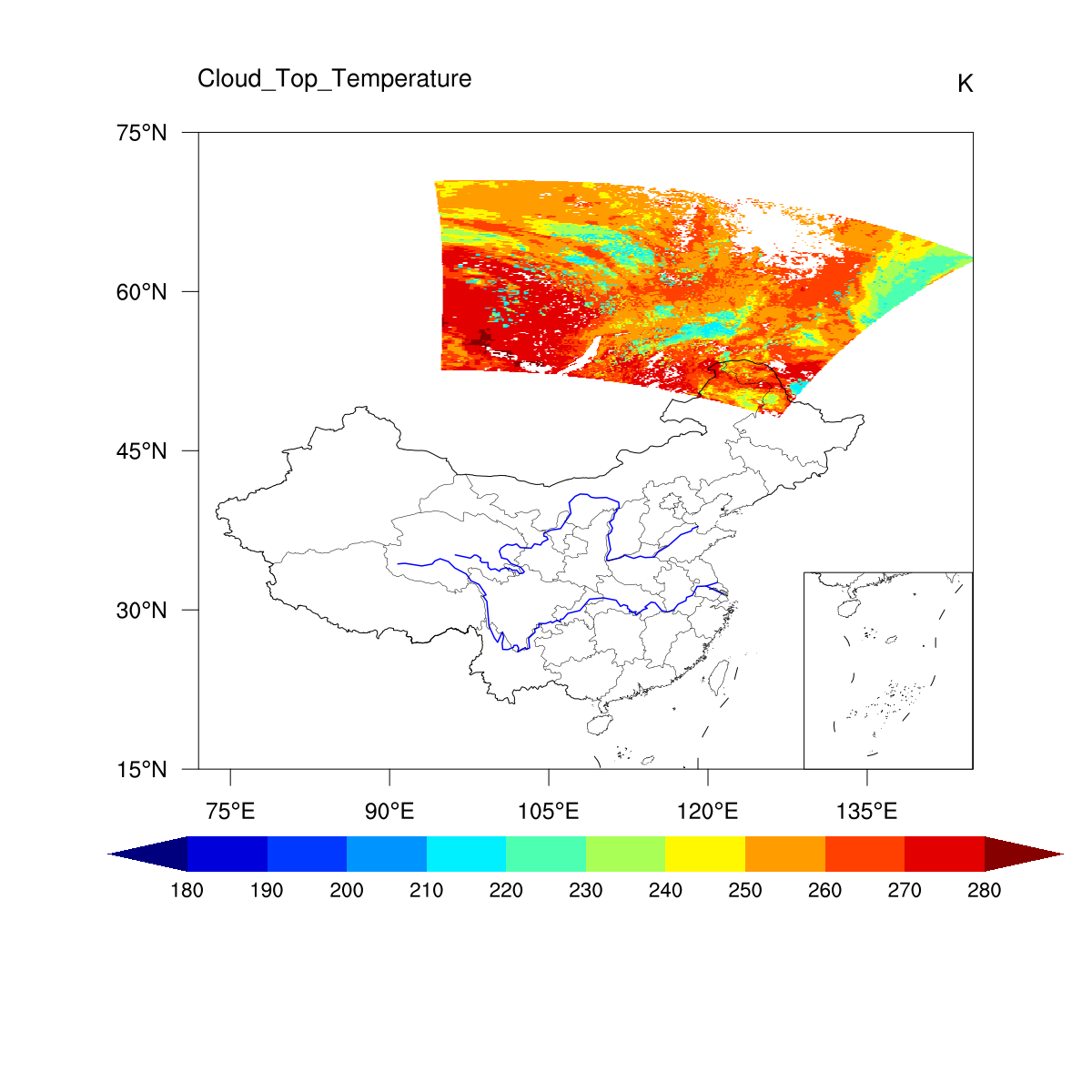
04.东亚区域MOD06_L2 Cloud_Top_Temperature原始数据绘图和脚本

1
2
3
4
5
6
7
8
9
10
11
12
13
14
15
16
17
18
19
20
21
22
23
24
25
26
27
28
29
30
31
32
33
34
35
36
37
38
39
40
41
42
43
44
45
46
47
48
49
50
51
52
53
54
55
56
57
58
59
60
61
62
63
64
65
66
67
68
69
70
71
72
73
74
75
76
77
78
79
80
81
82
83
84
85
86
87
88
89
90
91
92
93
94
95
96
97
98
99
100
101
102
103
104
105
106
107
108
109
110
111
112
113
114
115
116
117
118
119
120
121
122
123
124
125
126
127
128
129
130
131
132
133
134
135
136
137
138
139
140
141
142
143
144
145
146
147
148
149
150
151
152
153
154
155
156
157
158
159
160
161
162
163
164
165
166
167
168
169
170
171
172
173
174
175
176
177
178
179
180
181
182
183
184
185
186
187
188
189
190
191
192
193
194
195
196
197
198
199
200
201
202
203
204
205
; =============================================================================
; Author: Gavin | Affiliation: NJU
; Email : Zhpfu.atm@gmail.com
; Last modified: 2019-07-19 01:15
; Filename: MODIS_Full_Area_regrid_latlon2d_to_rectilinear_grid.ncl
; Description: Read MODIS data;
; Take TCC for example;
; Mapping to specific area;
; Plotting China area with China's nine-dash;
; Choosing different Map Projections;
; To Be Determined(TBD):
; 问题:需要局部微调,经纬度刻度最好四周都有;投影方式暂时只有圆柱等距投影
; Cylindrical Equidistant Projection;
; =============================================================================

; =============================================================================
; Given a start time and a title, this procedure calls get_cpu_time()
; to get the end_time, then prints "elapsed time" information.
; =============================================================================
procedure print_elapsed_time(start_time,title)
local end_time
begin

end_time = get_cpu_time()
print("======================================================================")
print(title + " elapsed time = " + (end_time-start_time) + " CPU seconds.")
print("======================================================================")
end

; =============================================================================
; ===================================MAIN======================================
; =============================================================================
start_time = get_cpu_time()

fpath = "/Users/zhpfu/Downloads/DATA_MAC/MODIS/Full_Area/"
fname = "MOD06_L2.A2016095.0340.061.2017326010830.hdf"

f1 = addfile(fpath+fname,"r")

lon2d = f1->Longitude(:,:)
lat2d = f1->Latitude(:,:)

; Set default value
; 65534 is the area out of Earth
lon2d@_FillValue = -999.9
lat2d@_FillValue = -999.9

if (any(ismissing(ndtooned(lon2d)))) then
print("Missing longitude coordinates detected")
end if

if (any(ismissing(ndtooned(lat2d)))) then
print("Missing latitude coordinates detected")
end if

; Set the specific area to plot
minlat = 15
maxlat = 75
minlon = 72
maxlon = 145

; Read cloud temperature.
wv1s = f1->Cloud_Top_Temperature


; Apply scale and offset and convert to double.
CTT0 = wv1s@scale_factor*1.d * (wv1s - wv1s@add_offset)
CTT0@_FillValue = -32768

; Add the attributes
lat2d@units = "degrees_north"
lon2d@units = "degrees_east"
CTT0@lat2d = lat2d
CTT0@lon2d = lon2d
CTT0@units = "K"
CTT0@coordinates = "lat2d lon2d"

print("++++++++++++++++AAAAA++++++++++++++++++")

; =============================================================================
; ================================plot=========================================
; =============================================================================

wks_type = "png"
wks_type@wkWidth = 2400
wks_type@wkHeight = 2400

wks = gsn_open_wks(wks_type,"MODIS_CTT_plot_China") ; send graphics to PNG file
gsn_define_colormap(wks, "NCV_jet") ;MPL_jet


res = True ; plot mods desired
res@gsnMaximize = True ; maximize plot in frame
res@gsnDraw = False
res@gsnFrame = False
res@gsnSpreadColors = True ; Use full color map

res@sfXArray = lon2d
res@sfYArray = lat2d


res@cnFillOn = True ; color fill
res@cnFillMode = "RasterFill" ; Raster mode is much faster
; res@cnRasterSmoothingOn = True
; res@cnFillPalette = "gui_default"
res@cnLinesOn = False ; and uses less memory.
res@cnLineLabelsOn = False
; res@trGridType = "TriangularMesh" ; Caution!!! can not ignore!

; =============================================================================
; set for map
res@mpLimitMode = "LatLon"
res@mpMinLatF = minlat
res@mpMaxLatF = maxlat
res@mpMinLonF = minlon
res@mpMaxLonF = maxlon

res@mpFillOn = True
res@mpDataSetName = "/Users/zhpfu/Downloads/DATA_MAC/FY_satellite/FY4A/NCL-Chinamap/database/Earth..4"
res@mpDataBaseVersion = "MediumRes" ; or "Ncarg4_1"
res@mpAreaMaskingOn = True
res@mpMaskAreaSpecifiers = (/"China","Japan", "North Korea","South Korea", "Russia"/)
res@mpOutlineSpecifiers = (/"China","China:Provinces"/)


res@mpLandFillColor = "white"
res@mpInlandWaterFillColor = "white"
res@mpOceanFillColor = "white"
res@mpFillBoundarySets = "NoBoundaries"
res@mpOutlineBoundarySets = "NoBoundaries"
res@mpNationalLineColor = "black"
res@mpProvincialLineColor = "black"
res@mpGeophysicalLineColor = "black"
res@mpNationalLineThicknessF = 2
res@mpProvincialLineThicknessF = 1

; =============================================================================
; set for the plot

res@cnFillDrawOrder = "PreDraw"
res@cnLevelSelectionMode = "ManualLevels" ; set manual contour levels
res@cnMinLevelValF = 180;min(olr) ; set min contour level
res@cnMaxLevelValF = 280;max(olr) ; set max contour level
res@cnLevelSpacingF = 10.0 ; set contour spacing

res@gsnAddCyclic = False

; res@tmXTOn = True
; res@tmYROn = True

res@lbOrientation = "Horizontal" ; vertical labelbar
res@pmTickMarkDisplayMode= "Always"
; res@pmLabelBarOrthogonalPosF = 0.00 ; Move labelbar up
; res@pmLabelBarParallelPosF = 0.00 ; Move labelbar Right
res@pmLabelBarWidthF = 0.65
res@pmLabelBarHeightF = 0.08
res@lbLabelFontHeightF = 0.018
res@lbPerimOn = False

res@lbLabelAutoStride = True ; Clean up labelbar labels.
res@lbBoxLinesOn = False ; No labelbar box lines.
res@lbLabelFontHeightF = 0.01 ; make labels smaller ( default=0.02 )
res@lbBoxEndCapStyle = "TriangleBothEnds" ; set the two-end triangle
res@tiXAxisString = ""
res@tiYAxisString = ""
res@gsnStringFontHeightF = 0.012
res@gsnLeftString = "Cloud_Top_Temperature"
res@gsnRightString = "K";"W/m2"

plot = gsn_csm_contour_map(wks,CTT0,res) ; create plot

; =============================================================================
; add South China Sea
nhres = res
nhres@gsnMaximize = False
nhres@vpHeightF = 0.18
nhres@vpWidthF = 0.18

nhres@mpMinLatF = 2
nhres@mpMaxLatF = 23
nhres@mpMinLonF = 105
nhres@mpMaxLonF = 123
nhres@lbLabelBarOn = False
nhres@tmXBOn = False
nhres@tmXTOn = False
nhres@tmYLOn = False
nhres@tmYROn = False
nhres@gsnLeftString = ""
nhres@gsnRightString = ""
map_nanhai = gsn_csm_contour_map(wks,CTT0,nhres)
adres = True
adres@amParallelPosF = 0.499 ; -0.5 is the left edge of the plot.
adres@amOrthogonalPosF = 0.50 ; -0.5 is the top edge of the plot.
adres@amJust = "BottomRight"
plotnh = gsn_add_annotation(plot,map_nanhai,adres)
; add Changjiang and Huanghe river
river = True
river@gsLineThicknessF = 3.0
river@gsLineColor = "blue"
plotrv = gsn_add_shapefile_polylines(wks,plot,"/Users/zhpfu/Downloads/DATA_MAC/FY_satellite/FY4A/NCL-Chinamap/cnmap_NetCDF/river.nc",river)
draw(plot)
frame(wks)

print_elapsed_time(start_time,"Plotting Over >>>>>>>")

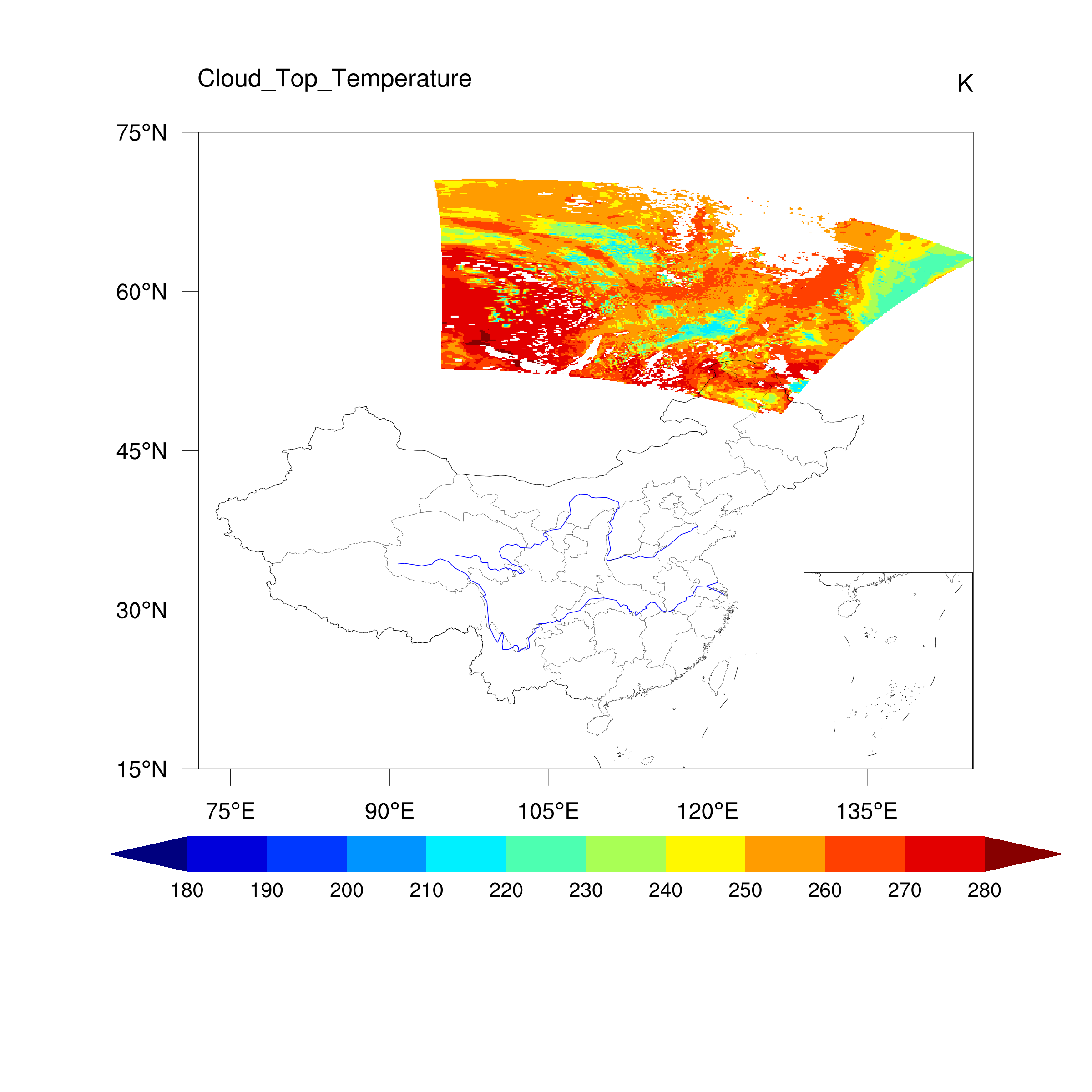
05.东亚区域MOD06_L2 Cloud_Top_Temperature插值数据绘图和脚本

1
2
3
4
5
6
7
8
9
10
11
12
13
14
15
16
17
18
19
20
21
22
23
24
25
26
27
28
29
30
31
32
33
34
35
36
37
38
39
40
41
42
43
44
45
46
47
48
49
50
51
52
53
54
55
56
57
58
59
60
61
62
63
64
65
66
67
68
69
70
71
72
73
74
75
76
77
78
79
80
81
82
83
84
85
86
87
88
89
90
91
92
93
94
95
96
97
98
99
100
101
102
103
104
105
106
107
108
109
110
111
112
113
114
115
116
117
118
119
120
121
122
123
124
125
126
127
128
129
130
131
132
133
134
135
136
137
138
139
140
141
142
143
144
145
146
147
148
149
150
151
152
153
154
155
156
157
158
159
160
161
162
163
164
165
166
167
168
169
170
171
172
173
174
175
176
177
178
179
180
181
182
183
184
185
186
187
188
189
190
191
192
193
194
195
196
197
198
199
200
201
202
203
204
205
206
207
208
209
210
211
212
213
214
215
216
217
218
219
220
221
222
223
224
225
226
227
228
229
230
231
232
233
234
235
236
237
238
239
240
241
242
243
244
245
246
247
248
249
250
251
252
253
254
255
256
257
258
259
260
261
262
263
264
265
266
267
268
269
270
271
272
273
274
275
276
277
278
279
280
281
282
283
284
285
286
287
288
289
290
291
292
293
294
295
296
297
298
299
300
301
302
303
304
305
306
307
308
309
310
311
312
313
314
315
316
317
318
319
320
321
322
323
324
325
326
327
328
329
330
331
332
333
334
335
336
337
338
339
340
341
342
343
344
345
346
347
348
349
350
351
352
353
354
355
356
357
358
359
360
361
362
363
364
365
366
367
368
; =============================================================================
; Author: Gavin | Affiliation: NJU
; Email : Zhpfu.atm@gmail.com
; Last modified: 2019-07-19 01:15
; Filename: MODIS_Full_Area_regrid_latlon2d_to_rectilinear_grid.ncl
; Description: Transform xy kilometer to lat lon grid;
; Output data with NetCDF;
; To Be Determined(TBD):
; 存在的问题是用rcm2rgrid_Wrap无法插值出有效的数值
; =============================================================================

; =============================================================================
; Given a start time and a title, this procedure calls get_cpu_time()
; to get the end_time, then prints "elapsed time" information.
; =============================================================================
procedure print_elapsed_time(start_time,title)
local end_time
begin

end_time = get_cpu_time()
print("======================================================================")
print(title + " elapsed time = " + (end_time-start_time) + " CPU seconds.")
print("======================================================================")
end

; =============================================================================
; ===================================MAIN======================================
; =============================================================================
load "$NCARG_ROOT/lib/ncarg/nclscripts/esmf/ESMF_regridding.ncl"

start_time = get_cpu_time()

fpath = "/Users/zhpfu/Downloads/DATA_MAC/MODIS/Full_Area/"
fname = "MOD06_L2.A2016095.0340.061.2017326010830.hdf"

f1 = addfile(fpath+fname,"r")

lon2d = f1->Longitude(:,:)
lat2d = f1->Latitude(:,:)

; Set default value
; 65534 is the area out of Earth
lon2d@_FillValue = -999.9
lat2d@_FillValue = -999.9

if (any(ismissing(ndtooned(lon2d)))) then
print("Missing longitude coordinates detected")
end if

if (any(ismissing(ndtooned(lat2d)))) then
print("Missing latitude coordinates detected")
end if

; Set the specific area to plot
minlat = 15
maxlat = 75
minlon = 72
maxlon = 145

; Read cloud temperature.
wv1s = f1->Cloud_Top_Temperature


; Apply scale and offset and convert to double.
CTT0 = wv1s@scale_factor*1.d * (wv1s - wv1s@add_offset)
CTT0@_FillValue = -32768

; Add the attributes
lat2d@units = "degrees_north"
lon2d@units = "degrees_east"
CTT0@lat2d = lat2d
CTT0@lon2d = lon2d
CTT0@units = "K"
CTT0@coordinates = "lat2d lon2d"

print("++++++++++++++++AAAAA++++++++++++++++++")

; Options to set for regridding
interp_method = "bilinear" ; Interpolation method: "bilinear" (default), "patch", or "conserve"

Opt = True
Opt@WgtFileName = "XY_to_rect.nc"

Opt@SrcGridLat = lat2d
Opt@SrcGridLon = lon2d

Opt@SrcRegional = True ; the default
Opt@SrcInputFileName = fpath+fname
Opt@DstRegional = True
Opt@SrcMask2D = where(.not.ismissing(CTT0),1,0) ; Necessary if has
; missing values.
Opt@InterpMethod = interp_method

Opt@DstGridType = "0.05deg" ; destination grid
Opt@DstTitle = "China Grid 0.05 degree resolution"
Opt@DstLLCorner = (/minlat, minlon/) ;;--Change (maybe)
Opt@DstURCorner = (/maxlat, maxlon/) ;;--Change (maybe)

print("++++++++++++++++BBBBB++++++++++++++++++")

Opt@ForceOverwrite = True
Opt@CopyVarCoords = True
Opt@Debug = True


CTT = ESMF_regrid(CTT0,Opt)
printVarSummary(CTT)
print("++++++++++++++++CCCCC++++++++++++++++++")


; ;---Interpolate to a 0.05x0.05 grid
; Opt = True
; Opt@ForceOverwrite = True
; Opt@Debug = True

; Opt@DstGridType = "0.05deg"
; Opt@WgtFileName = wgt_filename
; Opt@SrcMask2D = where(.not.ismissing(CTT),1,0)
; CTT = ESMF_regrid (CTT, opt)
; end if

; l3m_regrid@long_name = CTT@long_name + " (0.05x0.05)"


print("++++++++++++++++DDDDD++++++++++++++++++")
; =============================================================================
; Use the rcm2rgrid_Wrap to regridding
lat = new(1201 , "float",lat2d@_FillValue)
lon = new(1461, "float",lon2d@_FillValue)

lat = ispan(minlat*100,maxlat*100,5)*0.01
lon = ispan(minlon*100,maxlon*100,5)*0.01
lat@_FillValue = -999.9
lon@_FillValue = -999.9
; =============================================================================


lat@units = "degrees_north" ;don't forget to assign the LatLon attributes
lon@units = "degrees_east"
lat!0 = "lat"
lat&lat = lat
lon!0 = "lon"
lon&lon = lon

CTT!0 = "lat"
CTT&lat = lat
CTT!1 = "lon"
CTT&lon = lon
CTT@units = "K"
CTT@coordinates = "latlon"

printVarSummary(CTT)

print("Get subregional data!")
;===================================================================
; Assume variables T, PS and ORO exist and that they have
; associated meta data: (a) coordinate variables time, lev, lat, lon
; and (b) attributes
;===================================================================
nlat = dimsizes(lat)
nlon = dimsizes(lon)

filo = "CTT_China.nc" ; Output file
system("/bin/rm -f " + fpath + filo) ; remove if exists
fout = addfile (fpath + filo, "c") ; open output file

;===================================================================
; explicitly declare file definition mode. Improve efficiency.
;===================================================================
setfileoption(fout,"DefineMode",True)

;===================================================================
; create global attributes of the file
;===================================================================
fAtt = True ; assign file attributes
fAtt@title = "NCL Efficient Approach to netCDF Creation"
fAtt@source_file = ""
fAtt@Conventions = "None"
fAtt@creation_date = systemfunc ("date")
fileattdef( fout, fAtt ) ; copy file attributes

;===================================================================
; predefine the coordinate variables and their dimensionality
; Note: to get an UNLIMITED record dimension, we set the dimensionality
; to -1 (or the actual size) and set the dimension name to True.
;===================================================================
dimNames = (/"lat", "lon"/)
dimSizes = (/nlat, nlon/)
dimUnlim = (/False, False/)
filedimdef(fout,dimNames,dimSizes,dimUnlim)

;===================================================================
; predefine the the dimensionality of the variables to be written out
;===================================================================
; Here we are using NCL functions to facilitate defining
; each variable's dimension name(s) and type.
; The following could be replaced with explicit, user defined dimension
; names different from those associated with the variable in memory.
; Say, PS(time,lat,lon) in the NCL script. They could be redefined for the file via:
; filevardef(fout, "PS" ,typeof(PS) ,(/"TIME","latitude","longitude"/))
;===================================================================
filevardef(fout, "lat" ,typeof(lat) ,getvardims(lat))
filevardef(fout, "lon" ,typeof(lon) ,getvardims(lon))
filevardef(fout, "CTT" ,typeof(CTT) ,getvardims(CTT))

;===================================================================
; Copy attributes associated with each variable to the file
; All attributes associated with each variable will be copied.
;====================================================================
filevarattdef(fout,"lat" ,lat) ; copy lat attributes
filevarattdef(fout,"lon" ,lon) ; copy lon attributes
filevarattdef(fout,"CTT" ,CTT) ; copy CTT attributes
;===================================================================
; explicitly exit file definition mode. **NOT REQUIRED**
;===================================================================
setfileoption(fout,"DefineMode",False)

;===================================================================
; output only the data values since the dimensionality and such have
; been predefined. The "(/", "/)" syntax tells NCL to only output the
; data values to the predefined locations on the file.
;====================================================================
fout->lat = (/lat/)
fout->lon = (/lon/)
fout->CTT = (/CTT/)


; =============================================================================
; ================================plot=========================================
; =============================================================================

wks_type = "png"
wks_type@wkWidth = 2400
wks_type@wkHeight = 2400

wks = gsn_open_wks(wks_type,"MODIS_CTT_regrid_plot_China") ; send graphics to PNG file
gsn_define_colormap(wks, "NCV_jet") ;MPL_jet

; colors = (/ (/1,1,1/),\
; (/0,0,0/),\
; (/1,1,1/),\
; (/0.647,0.953,0.553/),\
; (/0.239,0.725,0.247/), \
; (/0.388,0.722,0.976/), \
; (/0,0,0.996/),\
; (/0.953,0.020,0.933/),\
; (/0.506,0,0.251/)/)

; gsn_define_colormap(wks,colors)


res = True ; plot mods desired
res@gsnMaximize = True ; maximize plot in frame
res@gsnDraw = False
res@gsnFrame = False
res@gsnSpreadColors = True ; Use full color map

; res@sfXArray = lon2d
; res@sfYArray = lat2d


res@cnFillOn = True ; color fill
res@cnFillMode = "RasterFill" ; Raster mode is much faster
; res@cnRasterSmoothingOn = True
; res@cnFillPalette = "gui_default"
res@cnLinesOn = False ; and uses less memory.
res@cnLineLabelsOn = False
; res@trGridType = "TriangularMesh" ; Caution!!! can not ignore!

; =============================================================================
; set for map
res@mpLimitMode = "LatLon"
res@mpMinLatF = minlat
res@mpMaxLatF = maxlat
res@mpMinLonF = minlon
res@mpMaxLonF = maxlon

res@mpFillOn = True
res@mpDataSetName = "/Users/zhpfu/Downloads/DATA_MAC/FY_satellite/FY4A/NCL-Chinamap/database/Earth..4"
res@mpDataBaseVersion = "MediumRes" ; or "Ncarg4_1"
res@mpAreaMaskingOn = True
res@mpMaskAreaSpecifiers = (/"China","Japan", "North Korea","South Korea", "Russia"/)
res@mpOutlineSpecifiers = (/"China","China:Provinces"/)


res@mpLandFillColor = "white"
res@mpInlandWaterFillColor = "white"
res@mpOceanFillColor = "white"
res@mpFillBoundarySets = "NoBoundaries"
res@mpOutlineBoundarySets = "NoBoundaries"
res@mpNationalLineColor = "black"
res@mpProvincialLineColor = "black"
res@mpGeophysicalLineColor = "black"
res@mpNationalLineThicknessF = 2
res@mpProvincialLineThicknessF = 1

; =============================================================================
; set for the plot

res@cnFillDrawOrder = "PreDraw"
res@cnLevelSelectionMode = "ManualLevels" ; set manual contour levels
res@cnMinLevelValF = 180;min(CTT) ; set min contour level
res@cnMaxLevelValF = 280;max(CTT) ; set max contour level
res@cnLevelSpacingF = 10.0 ; set contour spacing

res@gsnAddCyclic = False

; res@tmXTOn = True
; res@tmYROn = True

res@lbOrientation = "Horizontal" ; vertical labelbar
res@pmTickMarkDisplayMode= "Always"
; res@pmLabelBarOrthogonalPosF = 0.00 ; Move labelbar up
; res@pmLabelBarParallelPosF = 0.00 ; Move labelbar Right
res@pmLabelBarWidthF = 0.65
res@pmLabelBarHeightF = 0.08
res@lbLabelFontHeightF = 0.018
res@lbPerimOn = False

res@lbLabelAutoStride = True ; Clean up labelbar labels.
res@lbBoxLinesOn = False ; No labelbar box lines.
res@lbLabelFontHeightF = 0.01 ; make labels smaller ( default=0.02 )
res@lbBoxEndCapStyle = "TriangleBothEnds" ; set the two-end triangle
res@tiXAxisString = ""
res@tiYAxisString = ""
res@gsnStringFontHeightF = 0.012
res@gsnLeftString = "Cloud_Top_Temperature"
res@gsnRightString = "K";"W/m2"

plot = gsn_csm_contour_map(wks,CTT,res) ; create plot

; =============================================================================
; add South China Sea
nhres = res
nhres@gsnMaximize = False
nhres@vpHeightF = 0.18
nhres@vpWidthF = 0.18

nhres@mpMinLatF = 2
nhres@mpMaxLatF = 23
nhres@mpMinLonF = 105
nhres@mpMaxLonF = 123
nhres@lbLabelBarOn = False
nhres@tmXBOn = False
nhres@tmXTOn = False
nhres@tmYLOn = False
nhres@tmYROn = False
nhres@gsnLeftString = ""
nhres@gsnRightString = ""
map_nanhai = gsn_csm_contour_map(wks,CTT,nhres)
adres = True
adres@amParallelPosF = 0.499 ; -0.5 is the left edge of the plot.
adres@amOrthogonalPosF = 0.50 ; -0.5 is the top edge of the plot.
adres@amJust = "BottomRight"
plotnh = gsn_add_annotation(plot,map_nanhai,adres)
; add Changjiang and Huanghe river
river = True
river@gsLineThicknessF = 3.0
river@gsLineColor = "blue"
plotrv = gsn_add_shapefile_polylines(wks,plot,"/Users/zhpfu/Downloads/DATA_MAC/FY_satellite/FY4A/NCL-Chinamap/cnmap_NetCDF/river.nc",river)
draw(plot)
frame(wks)

print_elapsed_time(start_time,"Game Over >>>>>>>")

06.数据和脚本获取

公众号后台回复:“fy4a”

07.参考

链接.1
链接.2

有任何问题都欢迎交流探讨,共同学习进步!


-------------本文结束 感谢阅读-------------
作者Gavin
有问题请在相应页面留言(评论系统DISQUS需要"翻墙"才可见)
或者私信给我 GMAIL: zhpfu.atm@gmail.com
满分是10分的话,这篇文章你给几分
--> -->