Title:Improving Precipitation Estimation Using Convolutional Neural Network
标题:使用卷积神经网络改进降水估计
作者:Baoxiang Pan1, Kuolin Hsu1, Amir AghaKouchak1,2, and Soroosh Sorooshian1,2
1Center for Hydrometeorology and Remote Sensing, University of California, Irvine, CA, USA
2Department of Earth System Science, University of California, Irvine, CA, USA
期刊:Water Resources Research, 2019
Abstract:
Precipitation process is generally considered to be poorly represented in numerical weather/climate models. Statistical downscaling (SD) methods, which relate precipitation with model resolved dynamics, often provide more accurate precipitation estimates compared to model’s raw precipitation products. We introduce the convolutional neural network model to foster this aspect of SD for daily precipitation prediction. Specifically, we restrict the predictors to the variables that are directly resolved by discretizing the atmospheric dynamics equations. In this sense, our model works as an alternative to the existing precipitation‐related parameterization schemes for numerical precipitation estimation. We train the model to learn precipitation‐related dynamical features from the surrounding dynamical fields by optimizing a hierarchical set of spatial convolution kernels. We test the model at 14 geogrid points across the contiguous United States. Results show that provided with enough data, precipitation estimates from the convolutional neural network model outperform the reanalysis precipitation products, as well as SD products using linear regression, nearest neighbor, random forest, or fully connected deep neural network. Evaluation for the test set suggests that the improvements can be seamlessly transferred to numerical weather modeling for improving precipitation prediction. Based on the default network, we examine the impact of the network architectures on model performance. Also, we offer simple visualization and analyzing approaches to interpret the models and their results. Our study contributes to the following two aspects: First, we offer a novel approach to enhance numerical precipitation estimation; second, the proposed model provides important implications for improving precipitation‐related parameterization schemes using a data‐driven approach.
原文摘要:
通常情况下数值天气/气候模式中对于降水过程的描述是非常薄弱的环节。统计降尺度(SD)方法使得模式可解析的动力学过程与降水联系起来,就能够提供比模式初级产品更高精度的降水估计产品。我们引入了卷积神经网络模型来促进日降水预报的统计降尺度效果提升。尤其是我们限制了预报量为大气动力方程能离散解析的变量。从这个角度来讲,我们的模型可以替代现有的数值模式降水估计中的降水参数化方案。我们通过优化空间卷积核中的层级集合,来训练模型用于学习周围动力场中的降水关联的动力学特征。我们测试了横贯美国的14个地理格点。结果表明,提供足够的数据后,CNN模型的降水估计完胜再分析降水产品、线性回归的SD产品、最近相邻、随机森林,或者是全连通深度神经网络。评估测试集表明,这种提升能够无缝地移植到数值天气模式,并用于改进降水估计。基于默认的网络,我们检验了这种网络结构的模型性能方面。也就是,我们提供了简单的可视化和分析手段用于解释模型和其结果。我们研究主要有以下两方面的贡献:1.提供了新颖的方法用于数值模式降水估计;2.这种模型,使用了数据驱动方法对于改进降水关联的参数化方案有重要的意义。
图文
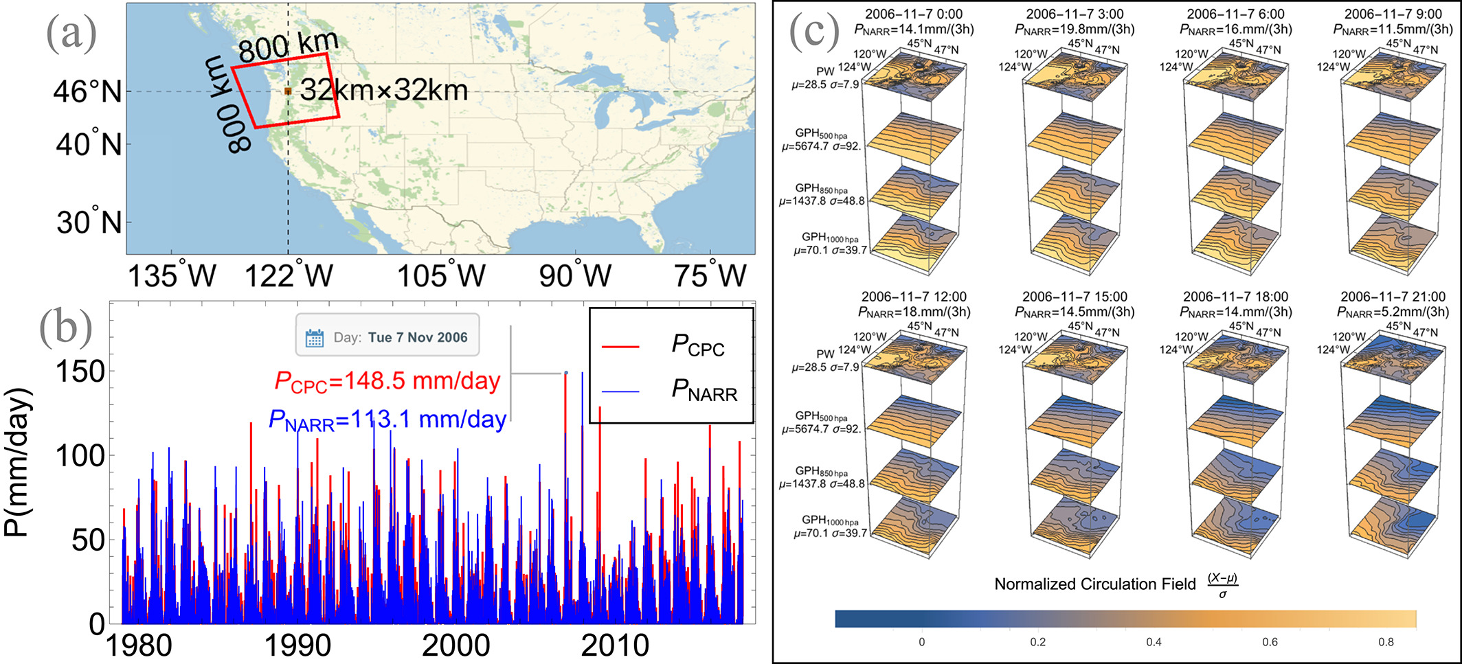
Figure 1, (a) The case study area of a 32 km × 32 km geogrid centered at 46°N, 122°W. Its surrounding circulation field is delineated with the 800 km × 800 km red polygon. (b) The geogrid’s daily precipitation time series from 1979 to 2017. The red thick line represents the gage‐based precipitation records from the National Oceanic and Atmospheric Administration Climate Prediction Center (CPC); the blue slim line represents the model reanalysis records from the National Centers for Environmental Prediction North American Regional Reanalysis Project (NARR). Data details are given in the section 5.1. (c) The every 3‐hr snapshots of the circulation profile for the storm event that happened on 7 November 2006. The geopotential height (GPH) at 1,000, 850, and 500 hPa and the total column precipitable water are obtained form NARR. Data are normalized by subtracting the field mean (μ) and dividing by the field standard deviation (σ).
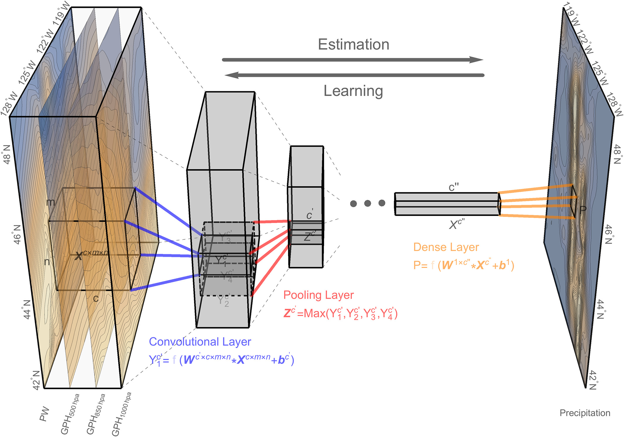
Figure 2, The convolutional neural network architecture for estimating precipitation using the numerical model resolved geopotential height and moisture field. The data are obtained from North American Regional Reanalysis Project data set. The stacked frames on the left side show the precipitable water (PW) and geopotential height (GPH) at 500, 850, and 1,000 hPa for the delineated 800 km×800 km region in Figure 1. The blue lines indicate a convolution operation applied on the circulation field. The red lines indicate the pooling operation that down‐samples the local features. Several stages of convolution and pooling layers are stacked, followed by the fully connected dense layers (orange lines). The dense layer applies all the extracted features to estimate precipitation for the target geogrid, which is labeled on the precipitation map on the right part. The convolution and dense layers are optionally followed by a nonlinear transformation f, which are represented with semitranslucent fonts.
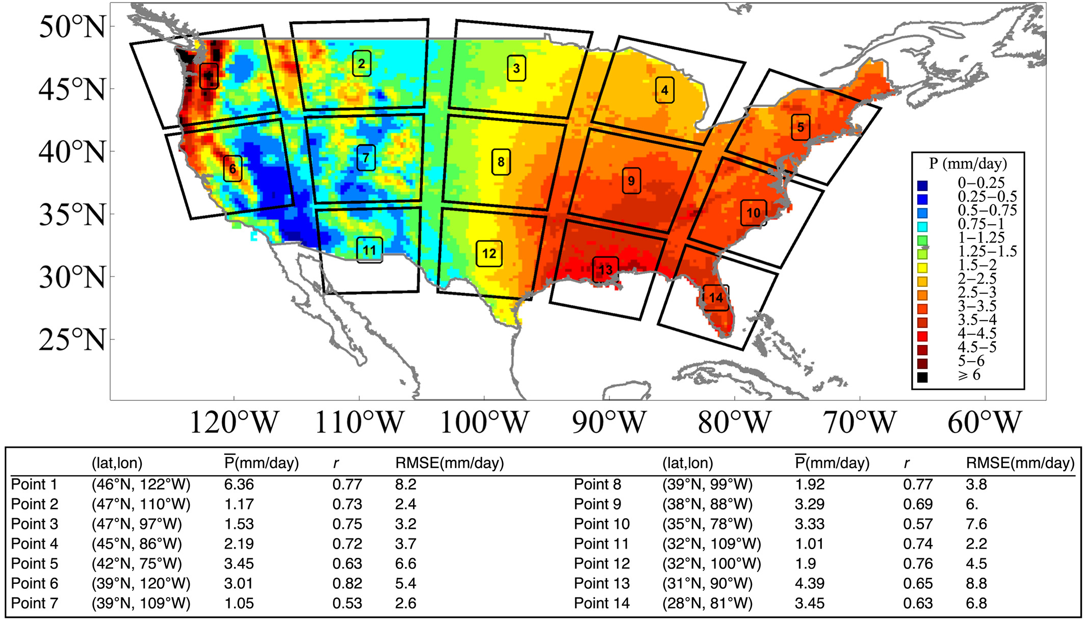
Figure 3, The sample grids used in the experiment. For each grid, the surrounding 800 km × 800 km dynamical field is delineated. The color indicates the mean daily precipitation rate, which is calculated by averaging the CPC daily precipitation records from 1979 to 2017. The table shows the samples’ coordinates, mean precipitation rate, the r, and root mean square error (RMSE) between North American Regional Reanalysis Project and Climate Prediction Center precipitation for the grids.
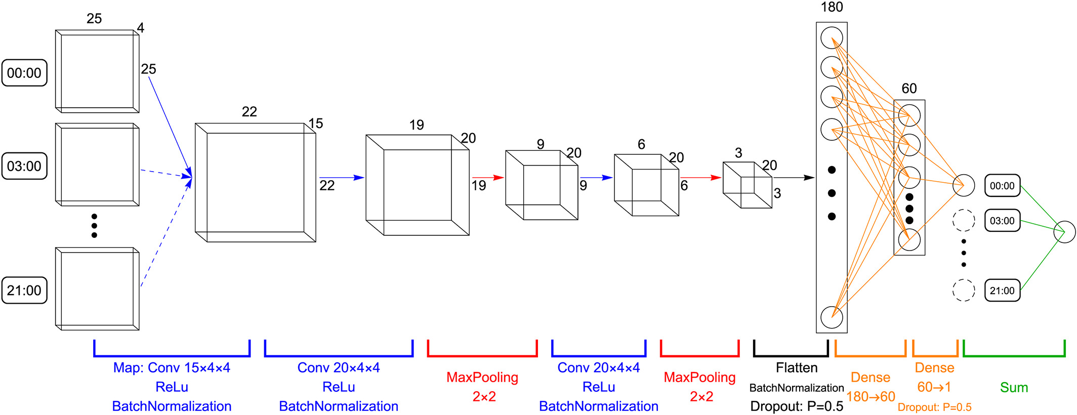
Figure 4, The network structure for precipitation estimation. Each 3‐hr snapshot of the dynamical field, which is represented by a 4 ×25× 25 tensor, is sequentially processes through the convolutional and pooling layers. The extracted features are flattened and processes by two consecutive dense layers. The dimension of each layer’s output is labeled out. Different layers/operators are denoted with corresponding colors. Results for eight 3‐hr snapshots are summed as the total daily precipitation estimate. In total, this network consists of 24,076 parameters to be trained.
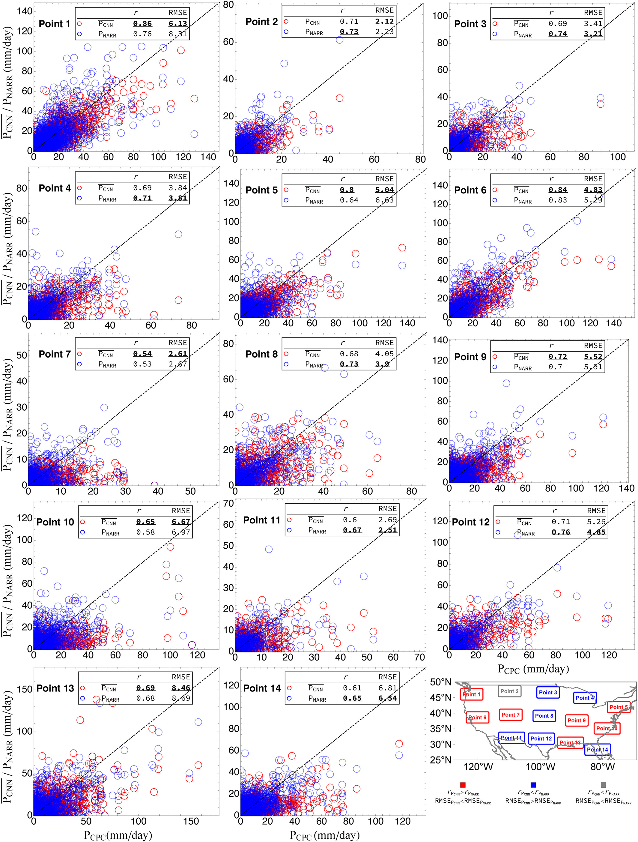
Figure 5, The scatter plots compare the urn:x-wiley:wrcr:media:wrcr23796:wrcr23796-math-0007 (red circles) /PNARR (blue circles) against the Climate Prediction Center precipitation records (Pobser) for the 14 sample points. Results are for the test set only. The skill scores of r and root mean square error (RMSE) for each point are given in corresponding subfigures. The bold and underlined value indicates the better statistics of the two estimates. The bottom right geographic map shows the geoposition of the 14 points. The point is labeled red/blue if both skill scores indicate that urn:x-wiley:wrcr:media:wrcr23796:wrcr23796-math-0008 / PNARR performs better. It is labeled gray if the two skill scores show disagreement. NARR = North American Regional Reanalysis Project; CNN = convolutional neural network.
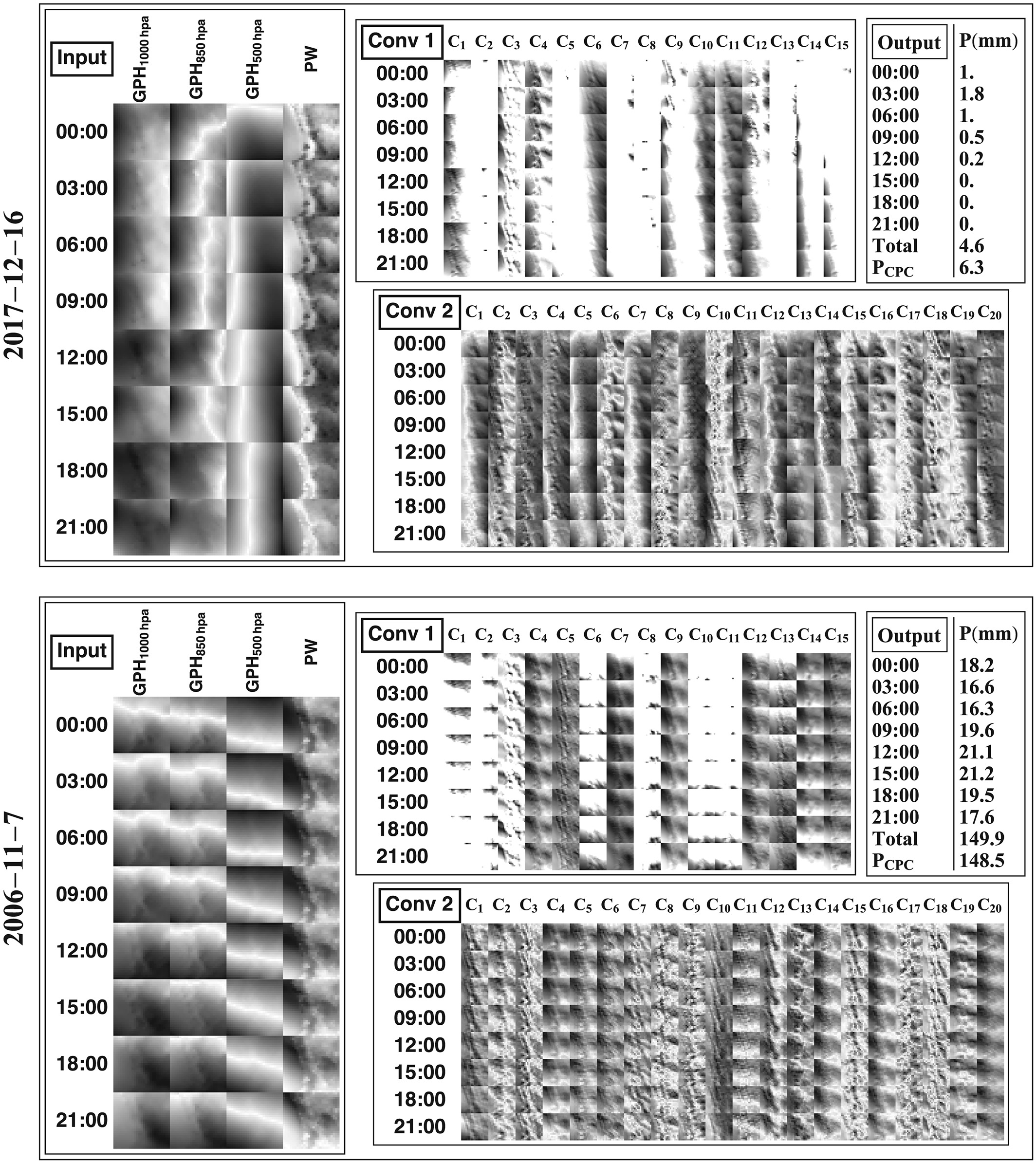
Figure 6, Layer activations for the 16 December 2017 light precipitation event (top) and 7 November 2006 storm event (bottom). The dark color represents low values, and bright color represents high values. The left part shows the eight 3‐hr snapshots of the dynamical field (GPH1,000 hPa, GPH850 hPa, GPH500 hPa, and PW) through the day. Conv 1/2 shows the activated output for the first/second convolutional layer. The Conv 1 result is composed of 8 × 15 subfigures. Eight indicates that there are eight 3‐hr dynamical field snapshots; 15 indicates that the output is of 15 channels, which are labeled as from C1 to C15. Similar denotations for Conv 2. The Output panel shows the results by mapping the convolutional neural network to each 3‐hr snap shot of the dynamical field. The sum of them consists the total daily precipitation estimate, which is compared against CPC records. PW = precipitable water; GPH = geopotential height.
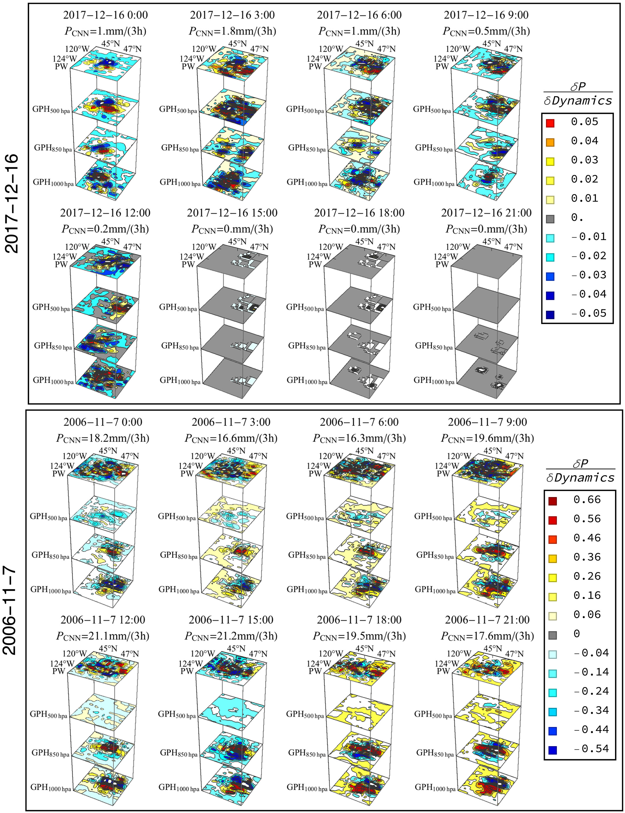
Figure 7, Perturbation sensitivity analysis for the 16 December 2017 light precipitation event (top) and 7 November 2006 storm event (bottom). For each case, we visualize the model output changes by systematically perturbing different portions of the scene with a rescaling matrix that is of same dimension as the first convolutional layer receptive field. The perturbation magnitude is set to 5%. The results are denoted as urn:x-wiley:wrcr:media:wrcr23796:wrcr23796-math-0115. We provide clear 2‐D projections of these figures in the supporting information. GPH = geopotential height; CNN = convolutional neural network.